1. Foundations of Time Series Regression
We often model a response \(Y_t\) as a linear function of a predictor \(X_t\) :
\[
\begin{align}
Y_t &= \beta_0 + \beta_1 X_t + \varepsilon_t, \\
\hat{\beta}_1 &= \frac{\sum (Y_t - \bar{Y})(X_t - \bar{X})}{\sum (X_t - \bar{X})^2}.
\end{align}
\]
Where:
\(Y_t\) is the response at time \(t\) .\(X_t\) is the predictor at time \(t\) .\(\beta_0\) is the intercept.\(\beta_1\) is the slope.\(\varepsilon_t\) is the error term.
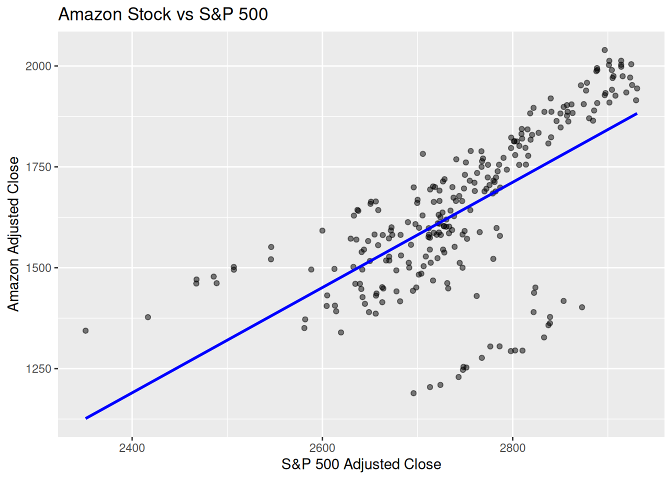
1.1 Finance Example (Amazon vs. S&P 500)
Dataset: gafa_stock (Amazon vs Market Index)
# 1) Get S&P 500 data (adjust as needed for start dates): <- tq_get ("^GSPC" , from = "2018-01-01" , to = "2019-12-31" ) %>% # Rename for consistency select (date, sp500_close = adjusted)# 2) Use Amazon data from gafa_stock in fpp3: <- gafa_stock %>% filter (Symbol == "AMZN" , Date >= "2018-01-01" , Date <= "2018-12-31" ) %>% select (Date, amzn_close = Adj_Close)# 3) Join by date <- amzn %>% inner_join (sp500, by = c ("Date" = "date" )) # Regression coefficients %>% model (TSLM (amzn_close ~ sp500_close)) %>% tidy () %>% :: kable (caption = "Coefficients table" )
Coefficients table
TSLM(amzn_close ~ sp500_close)
(Intercept)
-1940.961149
255.8360580
-7.586738
0
TSLM(amzn_close ~ sp500_close)
sp500_close
1.304591
0.0930976
14.013160
0
# 4) Quick visualization %>% ggplot (aes (x = sp500_close, y = amzn_close)) + geom_point (alpha = 0.5 ) + geom_smooth (method = "lm" , se = FALSE , color = "blue" ) + labs (title = "Amazon Stock vs S&P 500" ,x = "S&P 500 Adjusted Close" ,y = "Amazon Adjusted Close"
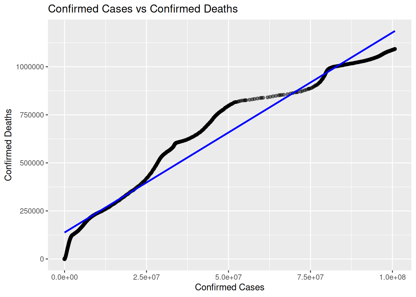
COVID Example (Mobility):
Dataset: oxcgrt (Oxford COVID Policy Tracker)
library (readr)<- "https://github.com/OxCGRT/covid-policy-dataset/raw/main/data/OxCGRT_compact_national_v1.csv" <- read_csv (url)
Model: \(\log(\text{ConfirmedCases}_t) = \beta_0 + \beta_1\text{ConfirmedDeaths}_t + \varepsilon_t\)
Activity: Test \(H_0: \beta_1=0\) using \(t = \frac{\hat{\beta}_1}{SE(\hat{\beta}_1)}\)
%>% filter (CountryName == "United States" ) %>% mutate (Date = lubridate:: ymd (Date)) %>% as_tsibble (index = Date) %>% :: drop_na (ConfirmedCases,ConfirmedDeaths ) %>% model (TSLM (ConfirmedCases ~ ConfirmedDeaths)) %>% tidy () %>% :: kable (caption = "Coefficients table" )
Coefficients table
TSLM(ConfirmedCases ~ ConfirmedDeaths)
(Intercept)
-1.054628e+07
4.288403e+05
-24.59255
0
TSLM(ConfirmedCases ~ ConfirmedDeaths)
ConfirmedDeaths
9.148213e+01
6.202599e-01
147.48998
0
<- oxcgrt %>% filter (CountryName == "United States" ) %>% mutate (Date = lubridate:: ymd (Date)) %>% as_tsibble (index = Date) %>% ggplot (aes (x = ConfirmedCases, y = ConfirmedDeaths)) + geom_point (alpha = 0.5 ) + geom_smooth (method = "lm" , se = FALSE , color = "blue" ) + labs (title = "Confirmed Cases vs Confirmed Deaths" ,x = "Confirmed Cases" ,y = "Confirmed Deaths"
Using oxdata for further COVID anaysis
Lab Activity 1
Filter the data to one country (e.g., ‘United States’).
Create a new variable, log_cases, defined as \(\\(\log(1 + \text{ConfirmedCases})\\)\) . (Adding 1 helps avoid \(\\(\log(0)\\).)\)
Fit a TSLM model relating log_cases to C6M_Stay at home requirements.
Interpret the slope coefficient.
Solution
# Filter & transform <- oxcgrt %>% filter (CountryName == 'United States' ) %>% mutate (Date = ymd (Date),log_cases = log (1 + ConfirmedCases)%>% as_tsibble (index = Date) %>% drop_na (log_cases, ` C6M_Stay at home requirements ` )# Fit TSLM <- exercise1_data %>% model (tslm_ex1 = TSLM (log_cases ~ ` C6M_Stay at home requirements ` ))# Summaries %>% tidy (tslm_ex1) %>% knitr:: kable ()
tslm_ex1
(Intercept)
14.976905
0.2302570
65.044305
0e+00
tslm_ex1
C6M_Stay at home requirements0.917216
0.1722268
5.325628
1e-07
%>% glance (tslm_ex1) %>% knitr:: kable ()
tslm_ex1
0.0252702
0.0243792
15.75292
28.36231
1e-07
2
-3065.006
3025.699
3025.721
3040.697
15.81785
17233.7
1094
2
Lab Activity 2
Filter to the same (or another) country.
Define a new variable, log_deaths = \(\\(\log(1 + \text{ConfirmedDeaths})\\)\) .
Regress log_deaths on StringencyIndex_Average using TSLM.
Check if increased stringency is correlated with reduced deaths (i.e., a negative slope).
Solution
# Filter & transform <- oxcgrt %>% filter (CountryName == 'United States' ) %>% mutate (Date = ymd (Date),log_deaths = log (1 + ConfirmedDeaths)%>% as_tsibble (index = Date) %>% drop_na (log_deaths, StringencyIndex_Average)# Fit TSLM <- exercise2_data %>% model (tslm_ex2 = TSLM (log_deaths ~ StringencyIndex_Average))# Summaries %>% tidy (tslm_ex2) %>% knitr:: kable ()
tslm_ex2
(Intercept)
9.3193169
0.2484414
37.51112
0
tslm_ex2
StringencyIndex_Average
0.0585671
0.0047442
12.34504
0
%>% glance (tslm_ex2) %>% knitr:: kable ()
tslm_ex2
0.1222721
0.1214698
9.854598
152.3999
0
2
-2807.946
2511.578
2511.6
2526.577
9.911232
10780.93
1094
2

