Activity50

# ----- Data Acquisition -----
fred_code <- "MRTSSM451211USN"
suppressMessages(getSymbols(fred_code, src = "FRED"))

[1] "MRTSSM451211USN"

book_sales_xts <- get(fred_code)

Time Series Analysis Framework

Trend Analysis

book_sales_tbl <- fortify.zoo(book_sales_xts) %>%
  rename(Date = Index, Sales = MRTSSM451211USN) %>%
  mutate(Month = yearmonth(Date)) %>%
  as_tsibble(index = Month)

book_sales_tbl %>%
  autoplot(Sales) +
  labs(y = "Sales (Millions of Dollars)", x = "Month") +
  theme_minimal(base_size = 12)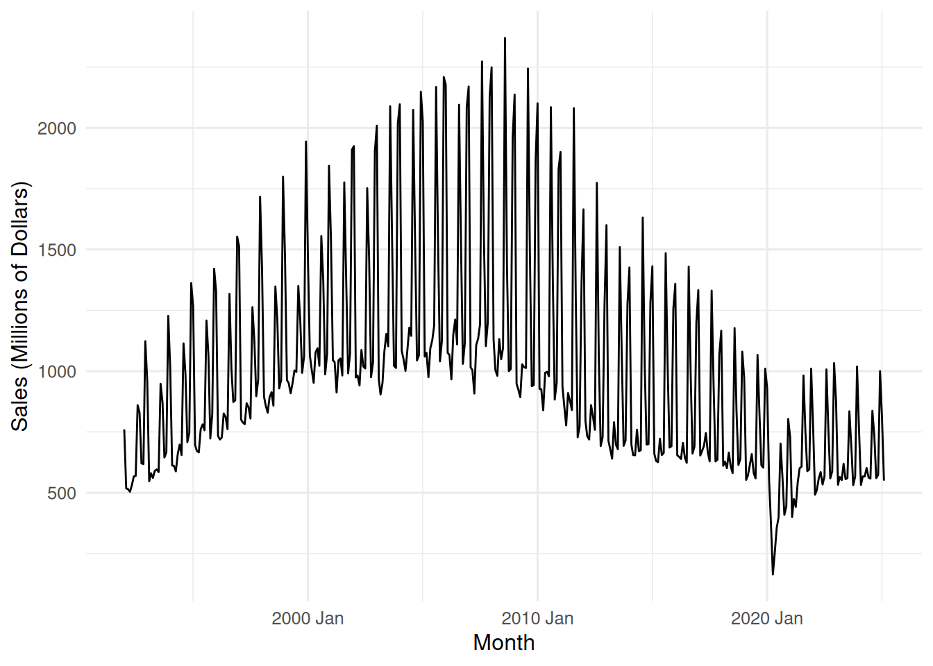

Monthly Retail Sales Trend: U.S. Book Stores

Seasonal Patterns

book_sales_tbl %>%
  gg_season(Sales, labels = "both") +
  labs(y = "Sales (Millions of Dollars)") +
  theme_minimal(base_size = 12)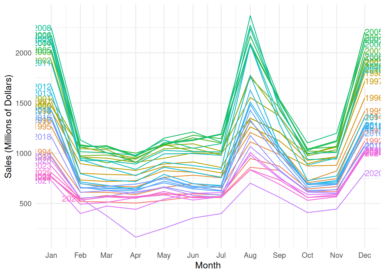

Seasonal Decomposition of Book Sales

Structural Decomposition

book_sales_tbl %>%
  model(STL(Sales ~ trend(window = 21) + season(window = "periodic"), robust = TRUE)) %>%
  components() %>%
  autoplot() +
  theme_minimal(base_size = 10)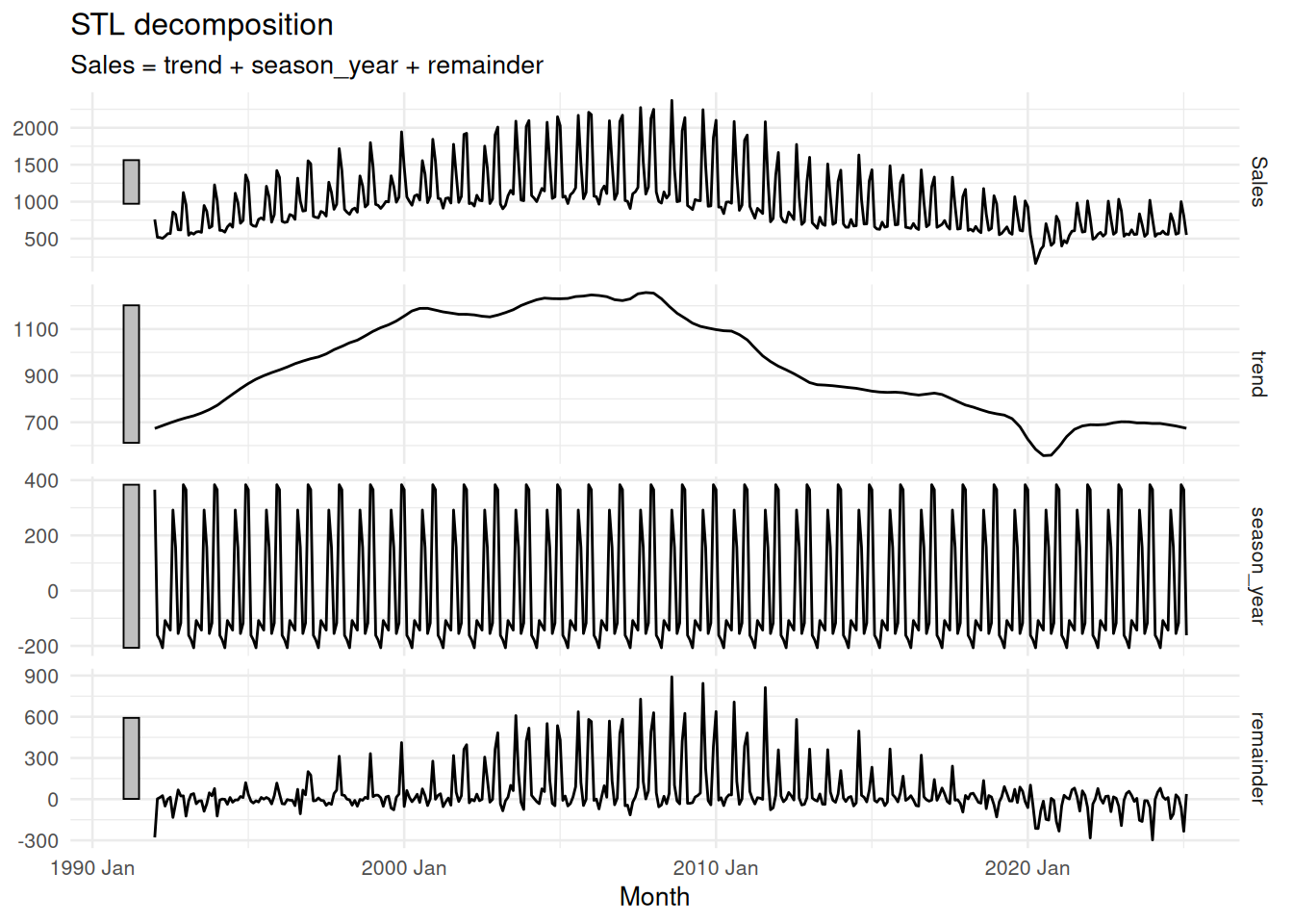

STL Decomposition of Sales Series

Modeling Results

ARIMA Diagnostics

arima_fit <- book_sales_tbl %>% model(ARIMA(Sales))
arima_fit %>% gg_tsresiduals()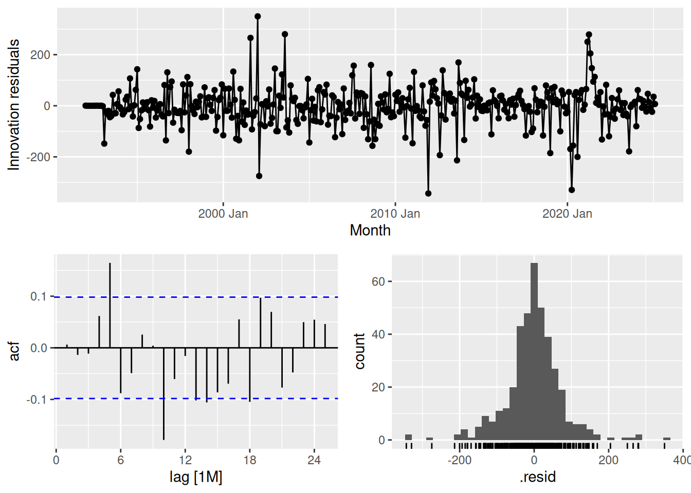 

ARIMA Model Residual Diagnostics

Box-Cox Transformation

lambda_est <- features(book_sales_tbl, Sales, guerrero)$lambda_guerrero
arima_fit_bc <- book_sales_tbl %>% model(ARIMA(box_cox(Sales, lambda_est)))
arima_fit_bc %>% gg_tsresiduals() 

Transformed Model Diagnostics

Exporting plots directly using chunk options

The following global configuration automates plot exports using knitr’s chunk options, standardizing all figures as 300dpi PNGs. By setting fig.path and dimensions globally, it ensures consistent output quality and organized file storage.

```{r chunk-export, include=FALSE}
# Global settings for all figures
knitr::opts_chunk$set(
  dev = "png",          # PNG device
  dpi = 300,            # Print quality
  fig.path = "figures/",# Organized storage
  fig.ext = "png",      # Explicit file extension
  fig.width = 8,        # 8" width
  fig.height = 4.5      # 4.5" height
)
```

Storing figures in a dedicated /figures folder maintains project organization for team workflows.

```{r main-plot, fig.cap="Book Sales Trend Analysis"}
# Plot will auto-save to figures/main-plot.png
book_sales_tbl %>%
  autoplot(Sales) +
  labs(title = NULL) +  # Titles in caption instead
  theme_minimal()
```

We can use knitr::include_graphics() to cleanly insert pre-saved PNGs into our markdown or presentation documents.

Embedding in Presentation

```{r embed-plot, echo=FALSE}
# Best practice inclusion method
knitr::include_graphics("figures/seasonal-plot.png")
```