Activity51

Ethical Considerations in Time Series Analysis

start_date <- "2010-01-01"
end_date <- Sys.Date() 

# Get data from Yahoo Finance
getSymbols("^GSPC", src = "yahoo", 
           from = start_date, 
           to = end_date, 
           auto.assign = TRUE) %>% invisible()

# Extract Adjusted Close prices and convert to tsibble
sp500_ts_scratch <- GSPC %>%
  Ad() %>% # Select Adjusted Close column
  `colnames<-`("Adjusted_Close") %>% # Rename column
  fortify.zoo(names = "Date") %>% # Convert zoo object to data frame
  as_tsibble(index = Date) %>%
  # Calculate log returns
  mutate(Log_Return = difference(log(Adjusted_Close))) %>%
  drop_na(Log_Return) %>% 
  fill_gaps(.full = TRUE) %>% 
  mutate(Log_Return = na.approx(Log_Return)) 

1. Data Integrity & Transparency

1.1 The Myth of Complete Data

Concept: All real-world time series contain gaps/imputation needs
Example: S&P 500 data:

sp500_ts <- GSPC %>%
  Ad() %>% 
  `colnames<-`("Adjusted_Close") %>%           # rename
  fortify.zoo(names = "Date") %>%              # to data.frame
  as_tsibble(index = Date) %>%                 # to tsibble
  fill_gaps() %>%                              # explicit missing days
  mutate(Adjusted_Close = na.approx(           # interpolate prices
    Adjusted_Close, rule = 2                   # rule=2: carry ends
  )) %>% 
  mutate(Log_Return = difference(log(Adjusted_Close))) 

sp500_ts_scratch <- GSPC %>%
  Ad() %>% # Select Adjusted Close column
  `colnames<-`("Adjusted_Close") %>% # Rename column
  fortify.zoo(names = "Date") %>% # Convert zoo object to data frame
  as_tsibble(index = Date) %>% 
  mutate(Log_Return = difference(log(Adjusted_Close))) 

Ethical Implications:

• 🚨 Silent imputation creates false continuity
• 📉 Hidden assumptions about market behavior
• 💡 Always report gap treatment methods (use imputeTS::na_ma() as alternative)

Visual Evidence:

sp500_ts_plot <- GSPC %>%
  Ad() %>%  `colnames<-`("Adjusted_Close") %>%           # rename
  fortify.zoo(names="Date") %>%
  as_tsibble(index=Date) %>%
  fill_gaps() %>%
  mutate(Log_Return = log(Adjusted_Close) - log(lag(Adjusted_Close)))

weekend_periods <- sp500_ts_plot %>%
  distinct(Date) %>%
  filter(wday(Date) %in% c(1,7)) %>%            # Sunday=1, Saturday=7
  arrange(Date) %>%
  mutate(grp = cumsum(c(1, diff(as.numeric(Date)) != 1))) %>%
  group_by(grp) %>%
  summarise(
    start = min(Date),                          # start at Sat midnight
    end   = max(Date) + days(1)                  # end at Mon midnight
  ) %>%
  ungroup()

library(scales)
ggplot(sp500_ts_plot, aes(Date, Log_Return)) +
  # (your weekend‐shade / rug / line layers here)  
  geom_rect(
    data = weekend_periods,
    aes(xmin = start, xmax = end, ymin = -Inf, ymax = Inf),
    inherit.aes = FALSE, fill = "grey80", alpha = 0.4
  ) +
  geom_line(color = "red", na.rm = TRUE) +
  
  # 1. Restrict x-axis to Jan 1 2023 – Feb 28 2023
  scale_x_date(
    limits     = as.Date(c("2023-01-01","2023-02-28")),
    date_breaks = "2 weeks",
    date_labels = "%b %d"
  ) +
  
  # 2. Force plain numeric y labels (no 1e-notation) with three decimals
  scale_y_continuous(
    labels = number_format(
      accuracy    = 0.001,
      big.mark     = ",",
      decimal.mark = "."
    )
  ) +
  
  labs(
    title = "S&P 500 Log-Returns (2023 Q1)",
    x     = NULL,
    y     = "Log Return"
  ) +
  theme_minimal()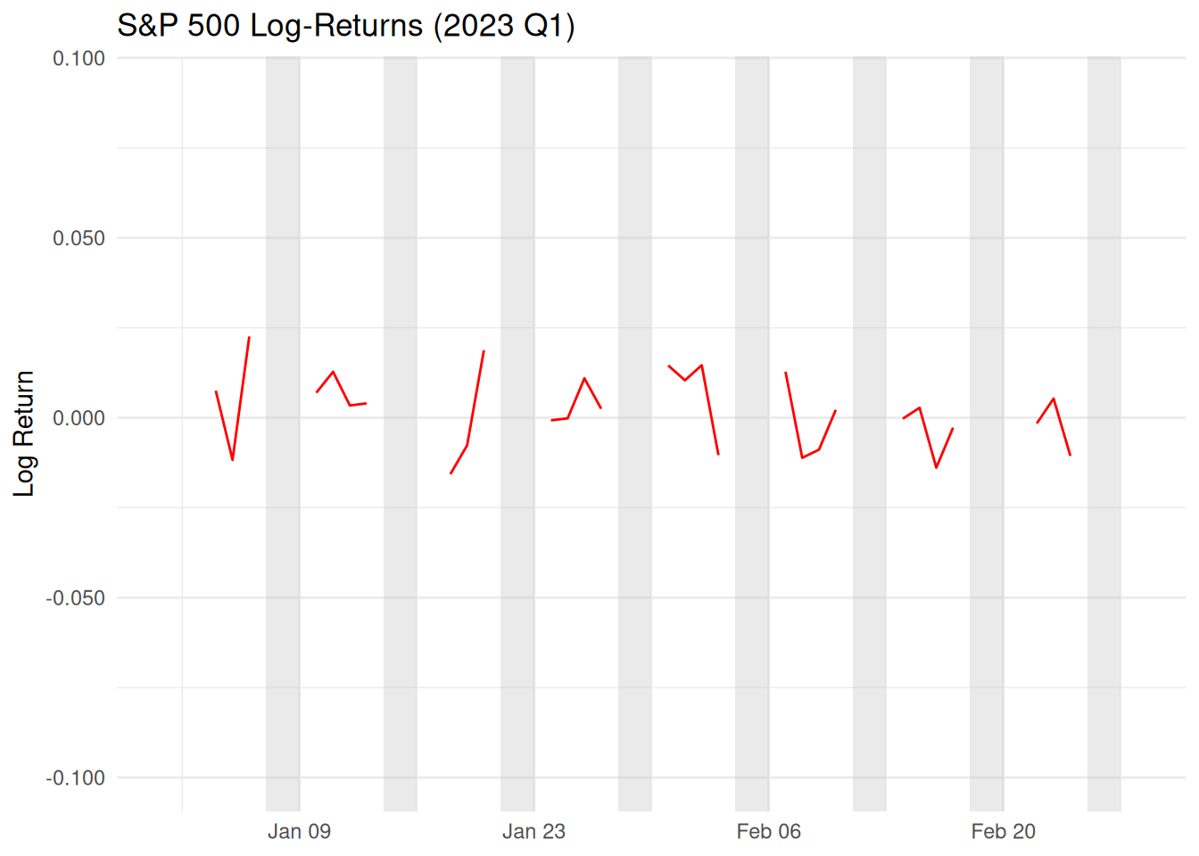

# --- Get US Unemployment Rate Data from FRED ---
start_date <- "1948-01-01"
end_date <- Sys.Date()

# Get data (UNRATE is the series ID for Civilian Unemployment Rate, Seasonally Adjusted)
getSymbols("UNRATE", 
           src = "FRED", 
           from = start_date, 
           to = end_date, 
           auto.assign = TRUE) %>% invisible()

# Convert to tsibble
unrate_ts <- UNRATE %>%
  fortify.zoo(names = "Date") %>% # Convert zoo to data frame
  # Ensure Date is Date class, create yearmonth index
  mutate(Month = yearmonth(Date)) %>%
  # Declare tsibble object
  as_tsibble(index = Month) %>%
  # Select relevant columns (rename UNRATE)
  select(Month, Unemployment_Rate = UNRATE)

1.2 Seasonality Manipulation

Concept: Seasonal adjustment choices impact policy decisions
Example: Unemployment Rate STL:

stl_decomp_unrate <- unrate_ts %>%
  model(  
    stl_decomp = STL(Unemployment_Rate ~ trend(window = 121) + 
                      season(window = "periodic"), 
                    robust = TRUE)
  ) %>%
  components()   

Ethical Risks:

• 🔍 Window size (121 months) smooths business cycles
• 📈 Different windows alter recession interpretations
• 💡 Document parameter sensitivity using fabletools::refit()

Visual Proof:

stl_decomp_unrate %>%
  autoplot() + 
  labs(subtitle="10-year Window Smoothing of Unemployment Trends")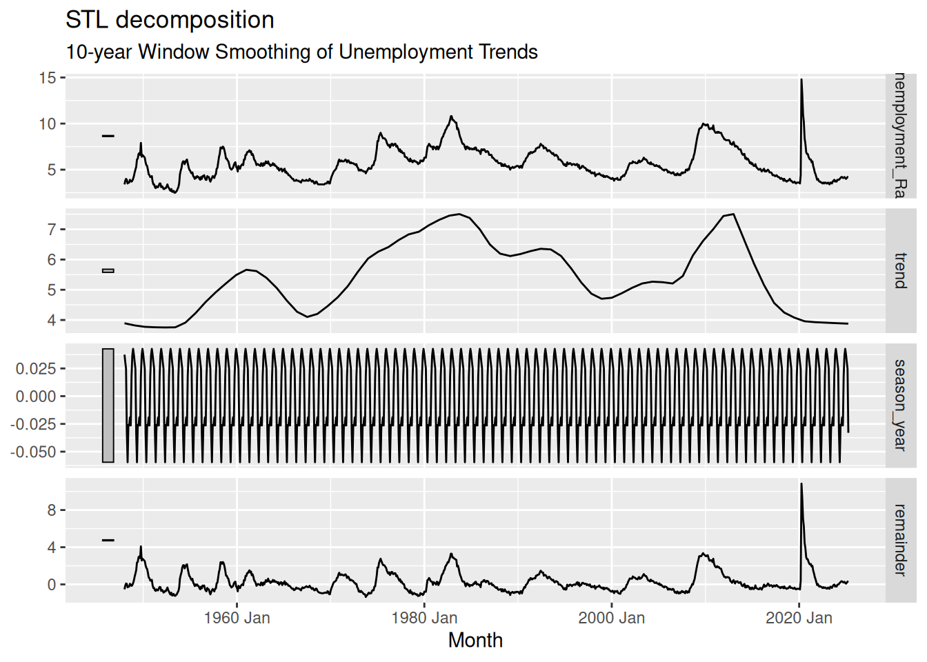

---

2. Model Accountability & Impact

2.1 Assumptions and Errors

Concept: Each transformation propagates errors
Case Study: Log Returns Pipeline:

library(imputeTS)
sp500_clean <- sp500_ts %>%
  # Remove non-trading days (weekends/holidays)
  filter(!is.na(Adjusted_Close)) %>%
  # Calculate log returns on valid trading days
  mutate(Log_Return = difference(log(Adjusted_Close))) %>%
  # Fill only actual trading day gaps (rare cases like exchange closures)
  fill_gaps(.full = FALSE) %>%
  # Ethical imputation with constraints
  mutate(
    Log_Return = na_locf(Log_Return, maxgap = 1) %>%  # Carry forward 1 day
    na_kalman() %>%                                   # State-space imputation
    na.omit()                                         # Remove leading NA
  )

Ethical Chain:

1. Logarithmic compression hides volatility scale
2. Linear interpolation assumes market continuity
3. Smoothing erases flash crash evidence
   Solution: Use imputeTS::na_kalman() for state-aware imputation

2.2 Non-Stationarity

Concept: Persistent series create false narratives
Unemployment ACF Analysis:

unrate_ts %>%  gg_tsdisplay(Unemployment_Rate, plot_type="partial")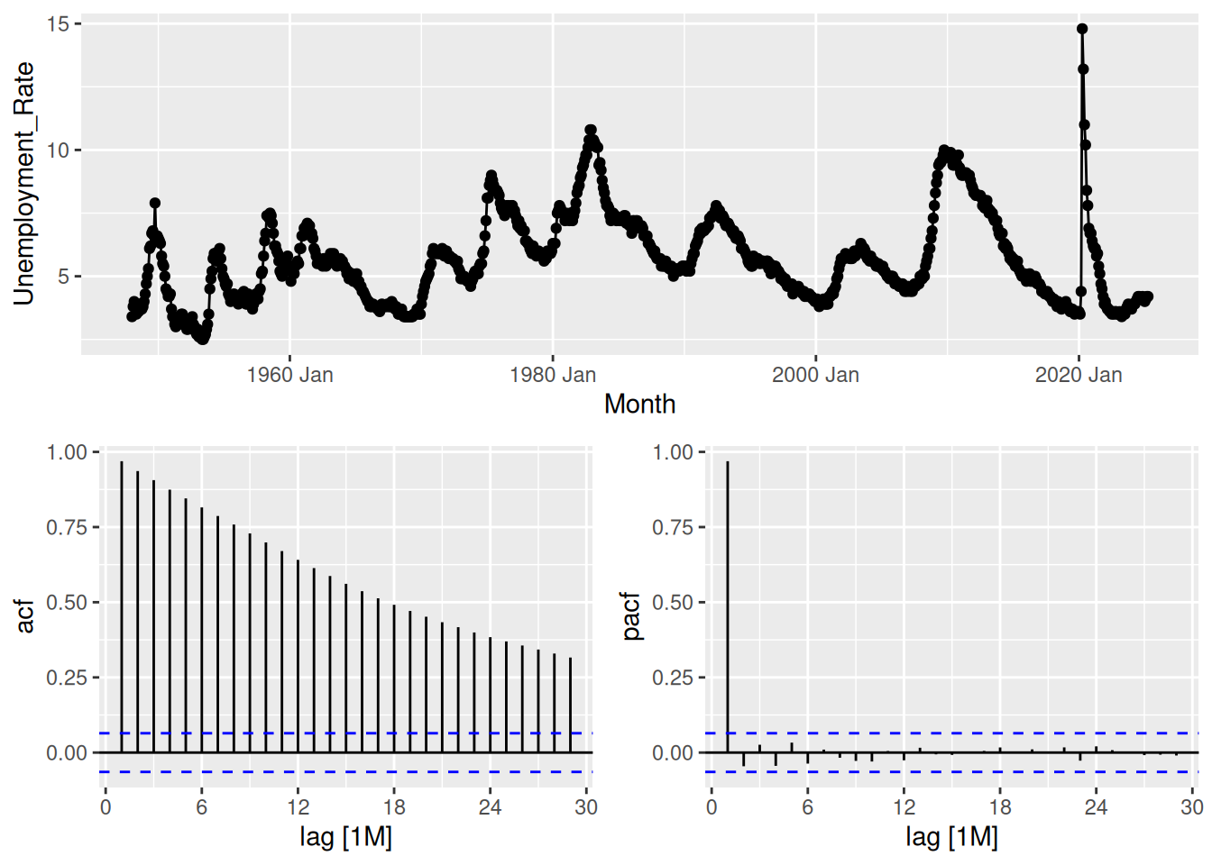

Dangers:

• Slow ACF decay (ρ₁=0.98) suggests structural persistence
• Mistaking hysteresis for mean-reversion
• 💣 Policy models might assume reversibility incorrectly

Remedies:

unrate_ts %>%
  features(Unemployment_Rate, unitroot_kpss) %>%
  knitr::kable(caption="Stationarity Test Results")

Stationarity Test Results

kpss_stat	kpss_pvalue
0.9870803	0.01

2.3 Temporal Aggregation Bias

Concept: Frequency choices shape narratives
Contrast:

# Daily vs Monthly Returns
sp500_daily <- sp500_ts %>% index_by(Date)
sp500_monthly <- sp500_ts %>% index_by(Month=yearmonth(Date)) %>%
  summarise(Volatility = sd(Log_Return, na.rm=TRUE))

Ethical Dimensions:

• 📅 Daily data shows volatility clusters
• 📆 Monthly aggregates hide flash crashes
• 💡 Use tsibble::index_by() consciously

Ethical Framework Checklist

ethical_checklist <- tibble(
  Step = c("Data Collection", "Gap Treatment", "Transformation",
           "Model Selection", "Interpretation"),
  Questions = c(
    "Source transparency?",
    "fill_gaps()/na.approx() documentation?",
    "Log/Sqrt transforms justified?",
    "Parameter sensitivity tested?",
    "Uncertainty intervals provided?")
)
knitr::kable(ethical_checklist)

Step	Questions
Data Collection	Source transparency?
Gap Treatment	fill_gaps()/na.approx() documentation?
Transformation	Log/Sqrt transforms justified?
Model Selection	Parameter sensitivity tested?
Interpretation	Uncertainty intervals provided?

Activities

Seasonality Manipulation & Model Sensitivity on us_employment

1.1 STL Window‐Choice and Its Policy Implications

# 1. Prepare series
empl_ts <- us_employment %>%
  filter(Title == "Total Private") %>%
  select(Month, Employed) %>%
  as_tsibble(index = Month)

# 2. Fit two STLs with different season windows
stl_short <- empl_ts %>% model(STL(Employed ~ trend(window=13) + season(window="periodic")))
stl_long  <- empl_ts %>% model(STL(Employed ~ trend(window=121) + season(window="periodic")))

decomp_short <- components(stl_short)
decomp_long  <- components(stl_long)

Tasks

1.  Plot the two trend components side by side (use autoplot(decomp_… , series="trend")).

2.  Overlay the original series with each smoothed trend to see how “cycle smoothing” differs.

3.  Discuss in writing:

•   How a 13-month vs 121-month window would affect decisions about recessions or stimulus timing.

•   Which choice feels more “transparent,” and what you’d need to report to a policymaker.

# 1. Side‐by‐side trend plots
trend_short <- decomp_short %>% select(Month, trend)
trend_long  <- decomp_long  %>% select(Month, trend)

p_short <- ggplot(trend_short, aes(Month, trend)) +
  geom_line() +
  labs(title="13-month STL Trend", y="Trend")

p_long <- ggplot(trend_long, aes(Month, trend)) +
  geom_line() +
  labs(title="121-month STL Trend", y="Trend")

library(gridExtra)
grid.arrange(p_short, p_long)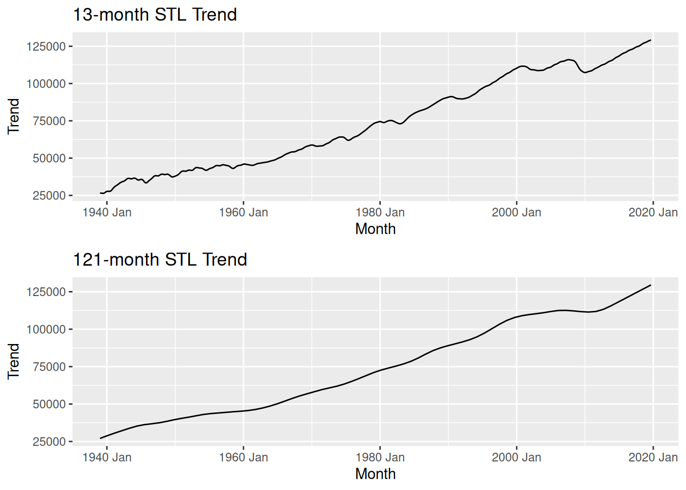

# 2. Overlay original series with both trends
empl_with_trends <- empl_ts %>%
  left_join(trend_short, by="Month") %>%
  rename(trend_short = trend) %>%
  left_join(trend_long,  by="Month") %>%
  rename(trend_long  = trend)

ggplot(empl_with_trends, aes(Month, Employed)) +
  geom_line(color="gray50") +
  geom_line(aes(y=trend_short), color="blue",  size=1) +
  geom_line(aes(y=trend_long),  color="red",   size=1) +
  labs(
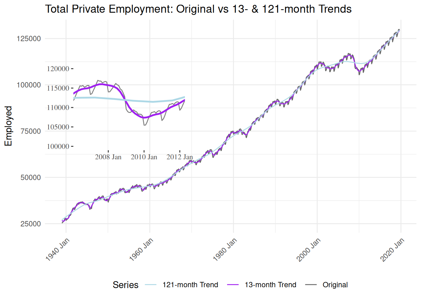
    title="Total Private Employment: Original vs 13- & 121-month Trends",
    y="Employed", x=NULL
  ) +
  theme_minimal()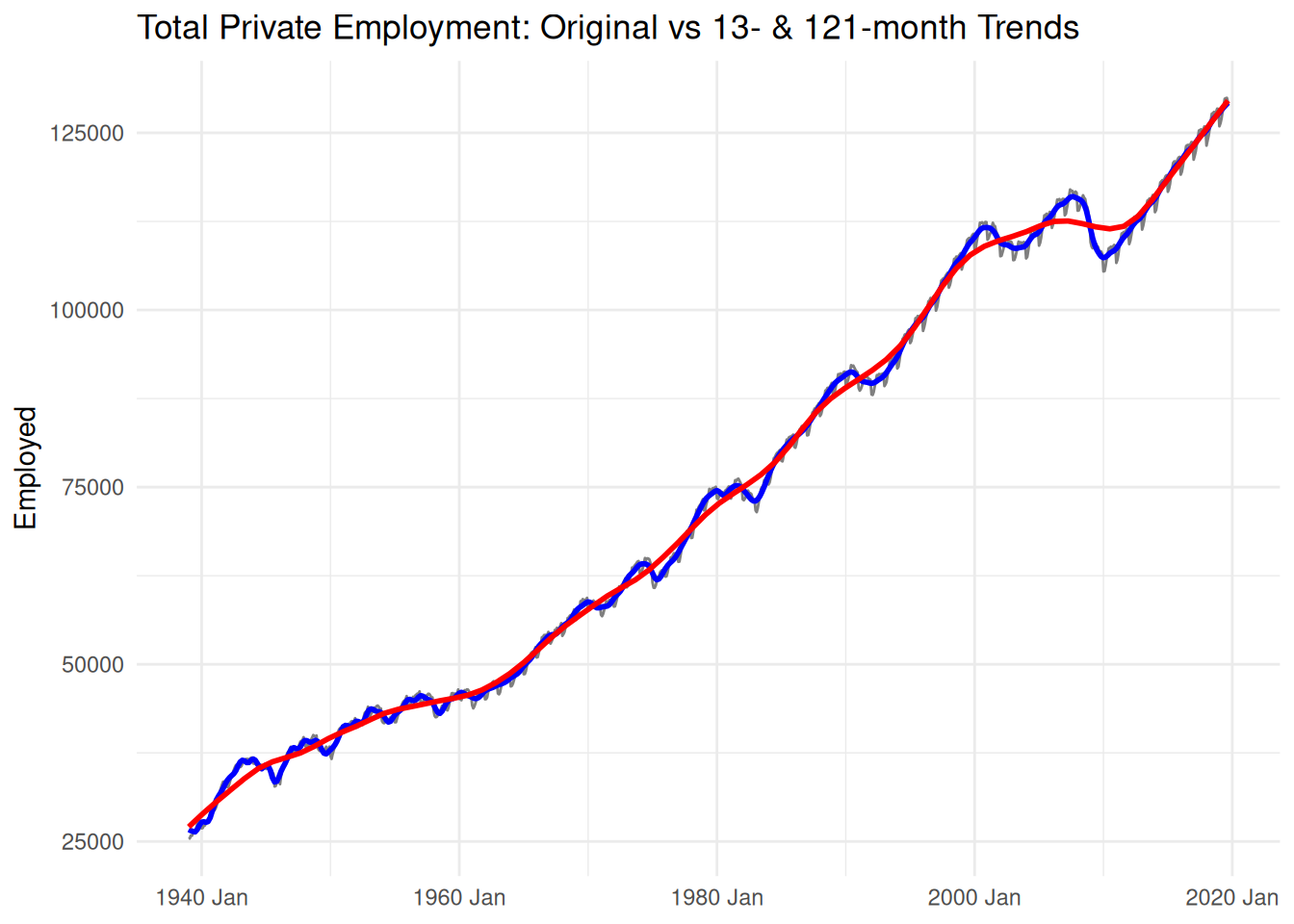

# Zoomed-in plot
ggplot(empl_with_trends, aes(Month, Employed)) +
  geom_line(color="gray50") +
  geom_line(aes(y=trend_short), color="blue",  size=1) +
  geom_line(aes(y=trend_long),  color="red",   size=1) +
  labs(
    title="Total Private Employment: Original vs 13- & 121-month Trends",
    y="Employed", x=NULL
  ) +
  coord_cartesian(xlim = yearmonth(c("1970 Jan", "1971 Jan"))) +
  scale_y_continuous(limits = c(55000, 60000))+
  theme_minimal()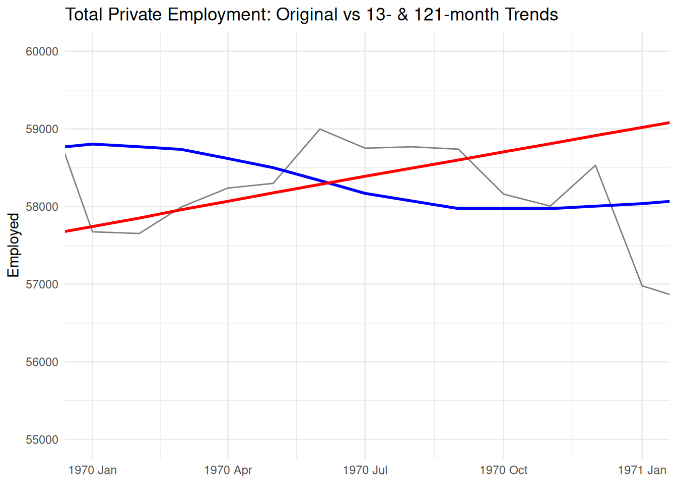

Overlaid plot

# 1. Full‐series plot
p_main <- ggplot(empl_with_trends, aes(x = Month)) +
  geom_line(aes(y = Employed,    color = "Original")) +
  geom_line(aes(y = trend_short, color = "13-month Trend")) +
  geom_line(aes(y = trend_long,  color = "121-month Trend")) +
  scale_color_manual(
    name   = "Series",
    values = c(
      "Original"        = "grey40",
      "13-month Trend"  = "purple",
      "121-month Trend" = "lightblue"
    )
  ) +
  labs(
    title = "Total Private Employment: Original vs 13- & 121-month Trends",
    y     = "Employed", x = NULL
  ) +
  theme_minimal() +
  theme(
    axis.text.x      = element_text(angle = 45, hjust = 1),
    legend.position  = "bottom",
    legend.direction = "horizontal"
  )

# 2. Zoomed‐in plot 
p_inset <- ggplot(empl_with_trends, aes(x = Month)) +
  geom_line(aes(y = Employed),    color = "grey50") +
  geom_line(aes(y = trend_short), color = "purple",    size = 1) +
  geom_line(aes(y = trend_long),  color = "lightblue", size = 1) +
  coord_cartesian(
    xlim = yearmonth(c("2006 May", "2012 Jan")),
    ylim = c(100000, 120000)
  ) +
  labs(x = NULL, y = NULL) +
  theme(
    legend.position = "none",
    axis.text.x = element_text(angle = 45, hjust = 1),
  ) + 
  ggthemes::theme_tufte()

# 3. Combine with cowplot
library(cowplot)
combined <- ggdraw() +
  draw_plot(p_main) +
  draw_plot(p_inset, x = 0.10, y = 0.45, width = 0.35, height = 0.35)

combined