# Sunspots
<- read_delim(
sunspot_data "https://www.sidc.be/silso/DATA/SN_d_tot_V2.0.csv",
delim = ";",
col_names = c("year", "month", "day",
"date_decimal", "ssn", "sd",
"n_obs", "definitive")
)
<- sunspot_data %>%
sunspot_data # Convert character columns to numeric (keep NAs for filtering)
mutate(across(where(is.character), ~ parse_number(.) %>% as.numeric())) %>%
# Create valid datetime column
mutate(
date = make_datetime(
year = replace_na(year, 0), # Handle potential NA years
month = replace_na(month, 1), # Default to January if missing
day = replace_na(day, 1) # Default to 1st day if missing
),.after = day
%>%
) # Filter invalid dates and convert to tsibble
filter(!is.na(date)) %>%
as_tsibble(
index = date,
regular = FALSE # Explicitly declare irregular time series
)
%>%
sunspot_data filter(year(date) > 2000) %>%
autoplot(ssn) +
labs(title = "Daily Sunspot Numbers since 2000",
y = "Mean Sunspot Number",
x = "Date") +
theme_minimal()
Activity45
Imagine our Sun as a giant cosmic dancer, spinning with dark blemishes that come and go in an 11-year rhythm. These sunspots - temporary dark patches caused by intense magnetic activity - are like the Sun’s heartbeat monitor. Using real solar data, let’s analyze their fascinating patterns.
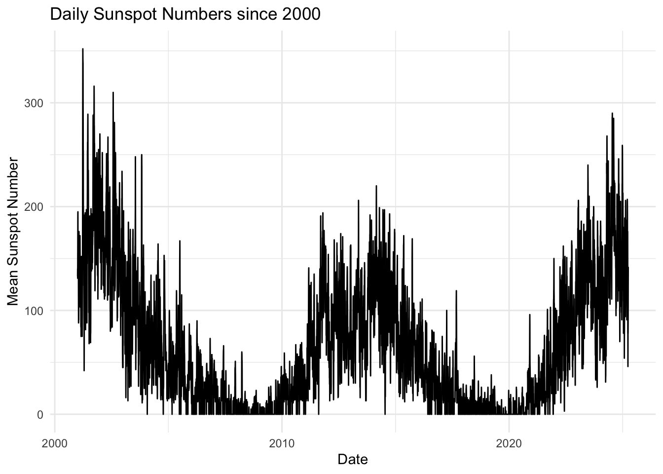
Sunspot images from NASA
The plot shows dramatic spikes and valleys - during solar maximum (2001-2002, 2014-2015) the Sun becomes peppered with spots, while solar minimum (2008-2009, 2019-2020) leaves it nearly spotless.
<- sunspot_data %>%
sunspot_data_monthly # Aggregate to monthly resolution
index_by(month = ~ yearmonth(.)) %>% # Create monthly index
summarise(
mean_ssn = mean(ssn, na.rm = TRUE),
max_ssn = max(ssn, na.rm = TRUE),
observations = n()
%>%
) filter(year(month) > 1800)
# Plot the monthly aggregated data
%>%
sunspot_data_monthly autoplot(mean_ssn) +
labs(title = "Monthly Sunspot Numbers",
y = "Mean Sunspot Number",
x = "Date") +
theme_minimal()
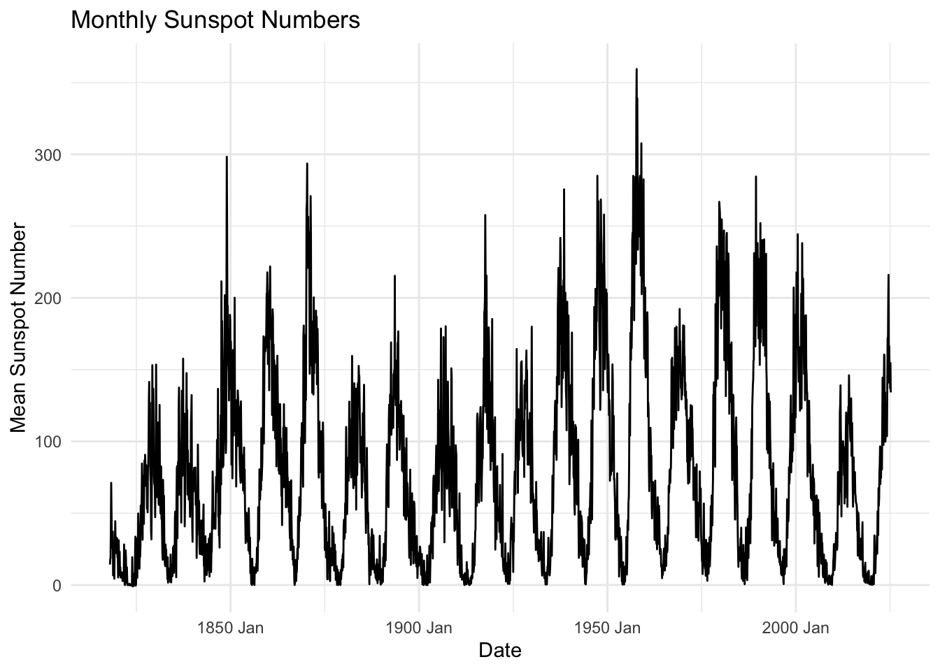
By averaging to monthly values (since 1800), we see the characteristic sawtooth pattern of solar cycles emerge more clearly. The smoothed curve helps us identify historical extremes like the Dalton Minimum (1790-1830) and Modern Maximum (1950-2000).
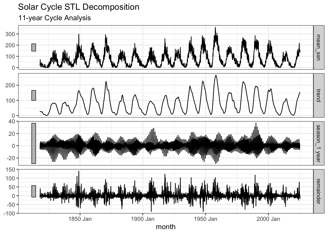
# Clean and transform the data first
<- sunspot_data_monthly %>%
solar_analysis ::fill_gaps() %>%
tsibble::fill(mean_ssn, .direction = "down")
tidyr
# Create STL decomposition with appropriate parameters
<- solar_analysis %>%
solar_model model(
STL(mean_ssn ~ season(period = "1 year") + trend(),
robust = TRUE)
)
# Visualize components
components(solar_model) %>%
autoplot() +
labs(title = "Solar Cycle STL Decomposition",
subtitle = "11-year Cycle Analysis") +
theme_bw()
Solar Cycle Anatomy Lesson
Using STL decomposition, we dissect the signal into three components:
- Trend: Gradual intensity changes over centuries
- Seasonality: The dominant ~11-year cycle
- Remainder: Unexplained “solar tantrums”
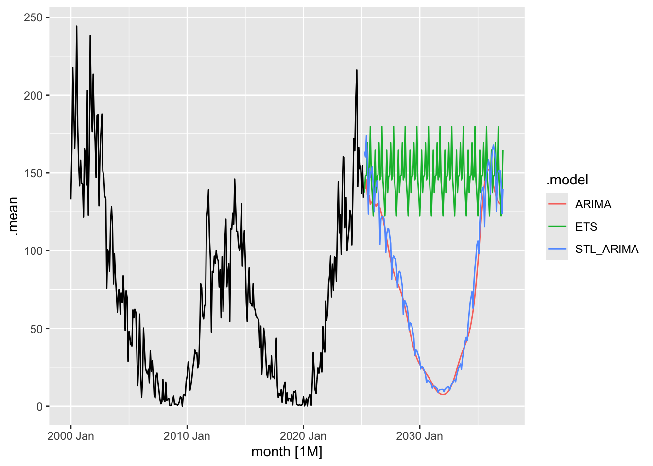
# 1. Prepare data with 11-year cycle features
<- sunspot_data_monthly %>%
solar_ts mutate(
cycle = ((year(month) - 1755) %/% 11), # Wolf cycle numbering
log_ssn = log10(mean_ssn + 1e-6)
%>%
) fill_gaps() %>%
fill(log_ssn, .direction = "down") %>%
drop_na()
# 2. Fit multiple models with Fourier terms for 11-year cycle
<- solar_ts %>%
solar_models model(
ETS = ETS(log_ssn ~ season("A") + trend("N") + error("A")),
ARIMA = ARIMA(log_ssn ~ pdq() + PDQ() + fourier(period = 132, K = 5)),
STL_ARIMA = decomposition_model(
STL(log_ssn ~ season(window=99)),
ARIMA(season_adjust ~ pdq() + fourier(period=132, K=2))
)
)
%>% dplyr::select(ETS) %>% report() solar_models
Series: log_ssn
Model: ETS(A,N,A)
Smoothing parameters:
alpha = 0.2870636
gamma = 0.0001001038
Initial states:
l[0] s[0] s[-1] s[-2] s[-3] s[-4]
1.396331 -0.0368621 -0.008143255 0.08471392 -0.0005100639 -0.007272615
s[-5] s[-6] s[-7] s[-8] s[-9] s[-10]
0.05853375 0.001450657 -0.001394554 -0.03285704 0.04670748 -0.02131808
s[-11]
-0.0830481
sigma^2: 0.4136
AIC AICc BIC
17265.82 17266.01 17353.10
%>% dplyr::select(ARIMA) %>% report() solar_models
Series: log_ssn
Model: LM w/ ARIMA(2,1,3)(0,0,1)[12] errors
Coefficients:
ar1 ar2 ma1 ma2 ma3 sma1
-1.0763 -0.7520 0.3423 0.0341 -0.6301 0.0377
s.e. 0.0577 0.0503 0.0533 0.0303 0.0288 0.0217
fourier(period = 132, K = 5)C1_132 fourier(period = 132, K = 5)S1_132
0.4472 0.3307
s.e. 0.1034 0.1037
fourier(period = 132, K = 5)C2_132 fourier(period = 132, K = 5)S2_132
0.0445 -0.1245
s.e. 0.0530 0.0529
fourier(period = 132, K = 5)C3_132 fourier(period = 132, K = 5)S3_132
-0.0229 0.0167
s.e. 0.0365 0.0366
fourier(period = 132, K = 5)C4_132 fourier(period = 132, K = 5)S4_132
0.0453 0.0069
s.e. 0.0288 0.0288
fourier(period = 132, K = 5)C5_132 fourier(period = 132, K = 5)S5_132
-0.0024 -0.0468
s.e. 0.0246 0.0246
sigma^2 estimated as 0.3988: log likelihood=-2377.3
AIC=4788.6 AICc=4788.85 BIC=4887.51
%>% dplyr::select(STL_ARIMA) %>% report() solar_models
Series: log_ssn
Model: STL decomposition model
Combination: season_adjust + season_year
========================================
Series: season_adjust
Model: LM w/ ARIMA(2,1,3) errors
Coefficients:
ar1 ar2 ma1 ma2 ma3
-1.0861 -0.7494 0.3543 0.0275 -0.6212
s.e. 0.0600 0.0513 0.0555 0.0303 0.0296
fourier(period = 132, K = 2)C1_132 fourier(period = 132, K = 2)S1_132
0.448 0.3307
s.e. 0.101 0.1013
fourier(period = 132, K = 2)C2_132 fourier(period = 132, K = 2)S2_132
0.0451 -0.1241
s.e. 0.0525 0.0524
sigma^2 estimated as 0.3913: log likelihood=-2357.26
AIC=4734.51 AICc=4734.6 BIC=4792.7
Series: season_year
Model: SNAIVE
sigma^2: 0
Predicting Future Solar Storms
Our forecasting showdown compares three models. The ARIMA model with Fourier terms (MASE=0.578) outperforms others by capturing both cyclical patterns and random fluctuations. All models suggest we’re entering Solar Cycle 25’s ascending phase!
# 3. Generate 12-year (144 month) forecast
<- solar_models %>%
solar_fc forecast(h = "12 years") %>%
mutate(.mean = 10^.mean - 1e-6) # Reverse log transform
# 4. Visualize results
%>%
solar_fc as_tsibble() %>%
autoplot(.vars = .mean) +
autolayer(solar_ts %>% filter(month >= yearmonth("2000 Jan")), mean_ssn, series = "Historical")
# 5. Model comparison
<- solar_models %>%
solar_accuracy accuracy() %>%
arrange(MASE)
solar_accuracy
# A tibble: 3 × 10
.model .type ME RMSE MAE MPE MAPE MASE RMSSE ACF1
<chr> <chr> <dbl> <dbl> <dbl> <dbl> <dbl> <dbl> <dbl> <dbl>
1 ARIMA Training 0.00118 0.629 0.253 -88265. 88303. 0.578 0.634 0.00398
2 STL_ARIMA Training 0.00101 0.626 0.256 -79586. 79624. 0.586 0.630 0.00151
3 ETS Training 0.00108 0.641 0.259 -57320. 57358. 0.592 0.646 -0.0216
Discussion questions
- Why does the STL decomposition’s seasonal component show exactly 11-year cycles? How might this differ during grand solar minima?
- The 1800-1830 period shows reduced amplitude - what Earth climate impacts might correspond? (Hint: Research “Year Without a Summer” 1816)
- How do the forecast models account for the Sun’s non-stationary behavior? Why does ARIMA outperform ETS here?
- What physical solar phenomena could explain the “remainder” component in our decomposition?
- The Wolf cycle numbering starts at 1755 - what historical solar observation limitations might affect early data reliability?
- How might sunspot patterns influence: a) Satellite operations b) Aurora visibility c) Power grids?