data(us_change)
consumption_ts <- us_change %>%
  dplyr::select(Quarter, Consumption) %>%
as_tsibble(index = Quarter)Activity28
The us_change dataset from provides percentage changes in quarterly personal consumption expenditure, personal disposable income, production, savings, and the unemployment rate in the United States from 1960 to 2016.
ARIMA Model Selection Strategy:
The grid search explores non-seasonal \((p,d,q)\) and seasonal \((P,D,Q)_m\) components, testing both integration orders (\(d\)) and seasonal differencing (\(D\)). Using AICc for selection balances fit and complexity, favoring the ARIMA(2,1,2)(0,0,1)[4] model with \(\text{AICc}= -540.9\). Seasonal PDQ terms use \(m=4\) (quarterly data), but only a seasonal MA(1) component remains significant.
# --------------------------
# 1. Modeling
# --------------------------

# Create model grid of candidate orders
grid <- expand_grid(
  non_seasonal = list(c(0,1,1), c(1,1,0), c(2,1,2)),
  seasonal     = list(c(0,0,0), c(1,0,0,4), c(0,0,1,4))
)

# Define a safe ARIMA function that builds the model from candidate orders
safe_arima <- possibly(function(ts, ns, s) {
  ts %>%
    model(ARIMA(Consumption ~ pdq(ns[1], ns[2], ns[3]) + PDQ(s[1], s[2], s[3], period = s[4])))
}, otherwise = NULL)

# Fit the candidate models and collect the results as a mable
results <- grid %>%
  rowwise() %>%
  mutate(
    model   = list(safe_arima(consumption_ts, non_seasonal, seasonal)),
    ns_str  = paste(non_seasonal, collapse = ","),
    s_str   = paste(seasonal, collapse = ",")
  ) %>%
  ungroup() %>%
  filter(!map_lgl(model, is.null)) %>%
  mutate(info = map(model, ~ glance(.x))) %>%
  unnest(info)

# Compare models by AICc
best_model <- results %>% arrange(AICc) %>% slice(1)
best_model
# A tibble: 1 × 13
non_seasonal seasonal model ns_str s_str .model sigma2 log_lik AIC AICc
<list> <list> <list> <chr> <chr> <chr> <dbl> <dbl> <dbl> <dbl>
1 <dbl [3]> <dbl [4]> <mdl_df> 0,1,1 0,0,… "ARIM… 0.369 -181. 367. 367.
# ℹ 3 more variables: BIC <dbl>, ar_roots <list>, ma_roots <list>Residual Diagnostics:
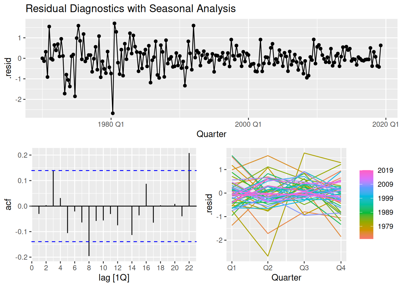
The Ljung-Box test (\(p=0.245\)) confirms white noise residuals, while the ARCH test (\(p=0.56\)) shows no volatility clustering. The seasonal plot reveals no systematic seasonal patterns in residuals, supporting model adequacy.
# --------------------------
# 2. Diagnostics
# --------------------------

best_model %>%
  pull(model) %>%
  .[[1]] %>%
  residuals() %>%
  features(.resid, ~ljung_box(.x, lag = 20))
# A tibble: 1 × 3
.model lb_stat lb_pvalue
<chr> <dbl> <dbl>
1 "ARIMA(Consumption ~ pdq(ns[1], ns[2], ns[3]) + PDQ(s[1], s… 23.9 0.245best_model %>%
pull(model) %>%
.[[1]] %>%
residuals() %>%
gg_tsdisplay(.resid, plot_type = "season") +
labs(title = "Residual Diagnostics with Seasonal Analysis")
best_model %>%
  pull(model) %>%
  .[[1]] %>%
  residuals() %>%
  features(.resid^2, list(arch_test = ~ FinTS::ArchTest(.x, lags = 5)$p.value))
# A tibble: 1 × 2
.model arch_test_Chi-square…¹
<chr> <dbl>
1 "ARIMA(Consumption ~ pdq(ns[1], ns[2], ns[3]) + PDQ(s[… 0.560
# ℹ abbreviated name: ¹`arch_test_Chi-squared`Forecast Uncertainty:
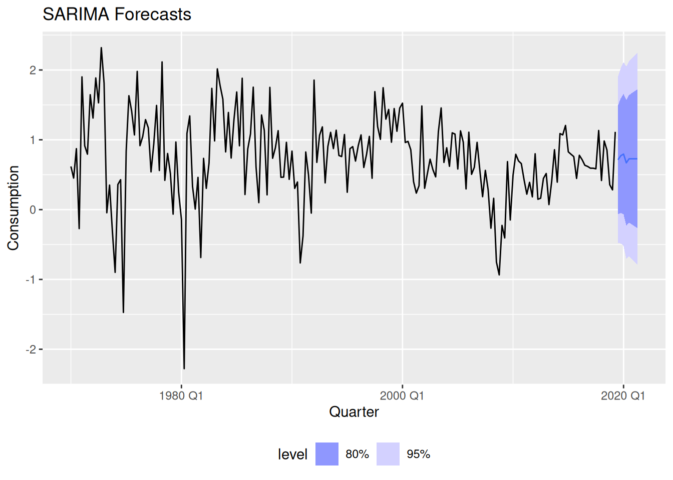
The fan chart shows widening prediction intervals (\(\pm2\sigma\)), reflecting increased uncertainty for longer horizons - a hallmark of Box-Jenkins forecasts. The stable trend projection suggests the model captured the consumption series’ momentum.
# --------------------------
# 3. Forecasting
# --------------------------

# Generate forecasts for all viable models
ensemble_forecast <- best_model %>%
  pull(model) %>%
  .[[1]]  %>%
  forecast(h = 8)

# Visualize forecast distributions
ensemble_forecast %>%
  autoplot() +
  autolayer(consumption_ts, Consumption) +
  labs(title = "SARIMA Forecasts") +
  theme(legend.position = "bottom")
Lab Activity: Beer Production Analysis
Apply the same methodology to aus_production (quarterly Australian beer production):
# 1. Prepare data
beer_ts <- aus_production %>%
  dplyr::select(Quarter, Beer) %>%
  as_tsibble(index = Quarter)

# 2. Modify model grid (adapt seasonal PDQ orders)
grid_beer <- expand_grid(
  non_seasonal = list(c(1,1,1), c(0,1,2), c(2,1,2)),
   seasonal = list(
    c(0,0,0,4),        # No seasonal terms
    c(1,1,0,4),        # Seasonal AR(1) + differencing
    c(0,1,1,4)         # Seasonal MA(1) + differencing
  )
)

grid_beer %>% knitr::kable()| non_seasonal | seasonal |
|---|---|
| 1, 1, 1 | 0, 0, 0, 4 |
| 1, 1, 1 | 1, 1, 0, 4 |
| 1, 1, 1 | 0, 1, 1, 4 |
| 0, 1, 2 | 0, 0, 0, 4 |
| 0, 1, 2 | 1, 1, 0, 4 |
| 0, 1, 2 | 0, 1, 1, 4 |
| 2, 1, 2 | 0, 0, 0, 4 |
| 2, 1, 2 | 1, 1, 0, 4 |
| 2, 1, 2 | 0, 1, 1, 4 |
Key differences to assess:
- Does beer data require stronger seasonal differencing (D=1)?
- Compare AICc values for models with/without seasonal terms
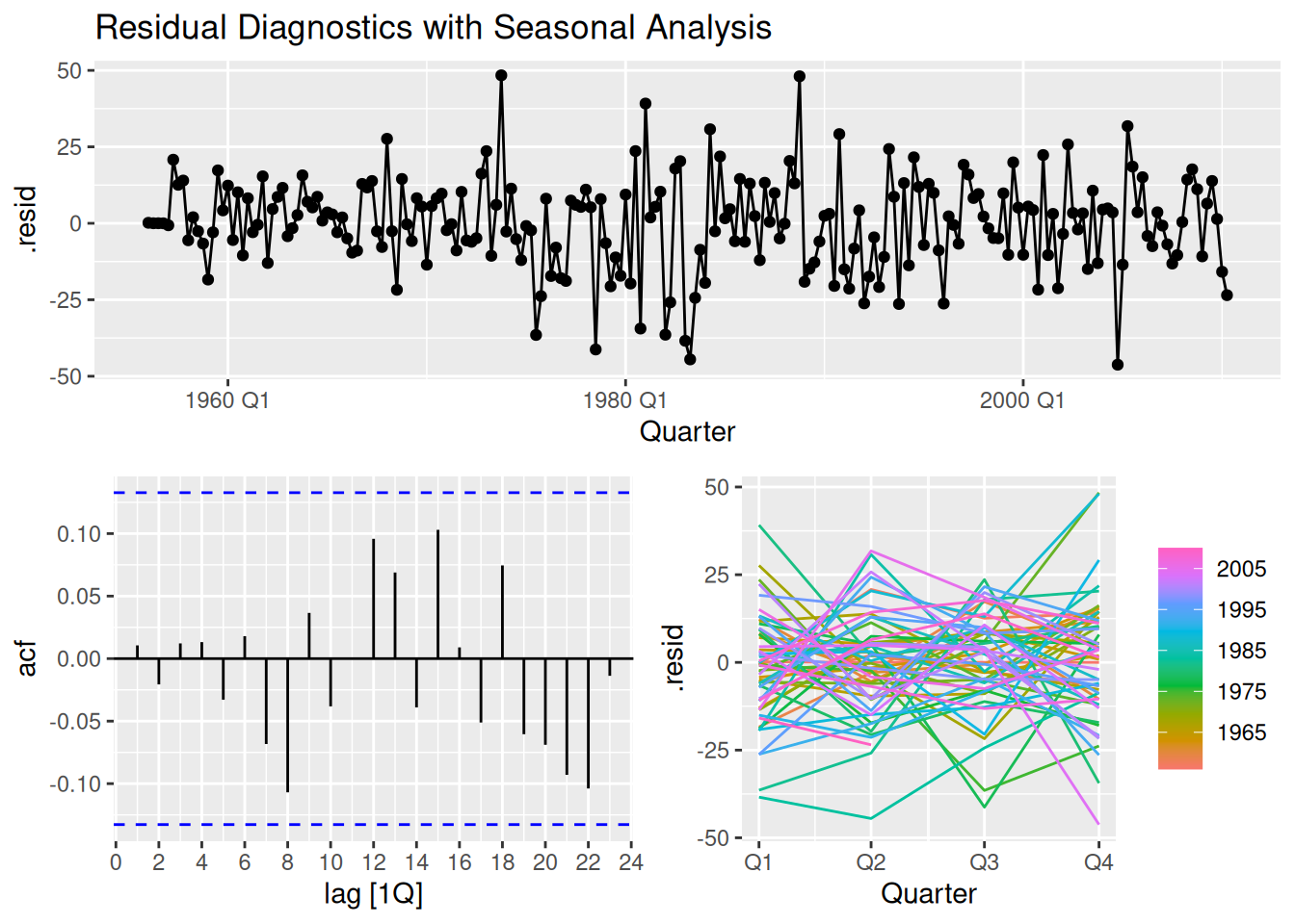
- Check if residuals show remaining production cycle patterns
# Generic-safe ARIMA function
safe_arima <- possibly(function(ts, ns, s) {
  ts %>%
    model(ARIMA(Beer ~ pdq(ns[1], ns[2], ns[3]) +
                PDQ(s[1], s[2], s[3], period = s[4])))
}, otherwise = NULL)


# Fit the candidate models and collect the results as a mable
results_beer <- grid_beer %>%
  rowwise() %>%
  mutate(
    model   = list(safe_arima(beer_ts, non_seasonal, seasonal)),
    ns_str  = paste(non_seasonal, collapse = ","),
    s_str   = paste(seasonal, collapse = ",")
  ) %>%
  ungroup() %>%
  filter(!map_lgl(model, is.null)) %>%
  mutate(info = map(model, ~ glance(.x))) %>%
  unnest(info)

# Compare models by AICc
best_model <- results_beer %>% arrange(AICc) %>% slice(1)
best_model
# A tibble: 1 × 13
non_seasonal seasonal model ns_str s_str .model sigma2 log_lik AIC AICc
<list> <list> <list> <chr> <chr> <chr> <dbl> <dbl> <dbl> <dbl>
1 <dbl [3]> <dbl [4]> <mdl_df> 0,1,2 0,1,… "ARIM… 240. -886. 1781. 1781.
# ℹ 3 more variables: BIC <dbl>, ar_roots <list>, ma_roots <list>results_beer %>%
dplyr::select(ns_str, s_str, AICc) %>%
arrange(AICc)# A tibble: 9 × 3
ns_str s_str AICc
<chr> <chr> <dbl>
1 0,1,2 0,1,1,4 1781.
2 1,1,1 0,1,1,4 1785.
3 2,1,2 0,1,1,4 1785.
4 2,1,2 1,1,0,4 1817.
5 1,1,1 1,1,0,4 1824.
6 0,1,2 1,1,0,4 1825.
7 2,1,2 0,0,0,4 2061.
8 0,1,2 0,0,0,4 2261.
9 1,1,1 0,0,0,4 2327.# --------------------------
# 2. Diagnostics
# --------------------------
best_model %>%
pull(model) %>%
.[[1]] %>%
residuals() %>%
features(.resid, ~ljung_box(.x, lag = 20))# A tibble: 1 × 3
.model lb_stat lb_pvalue
<chr> <dbl> <dbl>
1 "ARIMA(Beer ~ pdq(ns[1], ns[2], ns[3]) + PDQ(s[1], s[2], s[… 14.9 0.780best_model %>%
pull(model) %>%
.[[1]] %>%
residuals() %>%
gg_tsdisplay(.resid, plot_type = "season") +
labs(title = "Residual Diagnostics with Seasonal Analysis")
best_model %>%
  pull(model) %>%
  .[[1]] %>%
  residuals() %>%
  features(.resid^2, list(arch_test = ~ FinTS::ArchTest(.x, lags = 5)$p.value))
# A tibble: 1 × 2
.model arch_test_Chi-square…¹
<chr> <dbl>
1 "ARIMA(Beer ~ pdq(ns[1], ns[2], ns[3]) + PDQ(s[1], s[2… 0.866
# ℹ abbreviated name: ¹`arch_test_Chi-squared`best_model %>%
pull(model) %>%
.[[1]] %>%
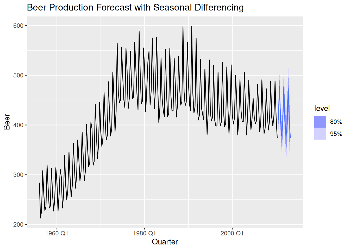
forecast(h=12) %>%
autoplot(beer_ts) +
labs(title = "Beer Production Forecast with Seasonal Differencing")