Columns: ['TIME', 'RATE', 'ERROR', 'YEAR', 'DAY', 'STAT_ERR', 'SYS_ERR', 'DATA_FLAG', 'TIMEDEL_EXPO', 'TIMEDEL_CODED', 'TIMEDEL_DITHERED']Activity48
The Crab Nebula is the remnant of the supernova observed in 1054 CE. It’s embedded Crab Pulsar, a rapidly rotating neutron star. The Crab Nebula is the expanding debris of SN 1054, located near ζ Tauri, and is one of the most intensively studied astronomical objects outside our Solar System. It lies about 2.0 kpc (≈6,500 ly) away and spans roughly 3.4 pc (≈11 ly), with its filaments racing outward at ~1,500 km/s—around 0.5% of light speed. At its heart spins the Crab Pulsar (PSR B0531+21), a six‑mile‑across neutron star rotating ∼30 times per second, whose strong magnetic field powers the nebula’s synchrotron emission. X‑ray observatories such as Swift/BAT and Chandra use the Crab as an in-flight calibration source because its high‑energy flux has remained remarkably stable over decades.
Rows: 5,759
Columns: 11
$ TIME             <dbl> 53414, 53416, 53419, 53420, 53421, 53422, 53423, 5342…
$ RATE             <dbl> 0.2186489, 0.2087431, 0.1986521, 0.1914362, 0.1904584…
$ ERROR            <dbl> 0.00788850, 0.00735829, 0.00721301, 0.00702885, 0.006…
$ YEAR             <dbl> 2005, 2005, 2005, 2005, 2005, 2005, 2005, 2005, 2005,…
$ DAY              <dbl> 44, 46, 49, 50, 51, 52, 53, 54, 61, 62, 64, 65, 67, 6…
$ STAT_ERR         <dbl> 0.00163894, 0.00074965, 0.00164370, 0.00181844, 0.001…
$ SYS_ERR          <dbl> 0.00765271, 0.00730601, 0.00695282, 0.00670027, 0.006…
$ DATA_FLAG        <dbl> 0, 0, 0, 0, 0, 0, 0, 0, 0, 0, 0, 0, 0, 0, 0, 0, 0, 0,…
$ TIMEDEL_EXPO     <dbl> 832, 4000, 5632, 2536, 2752, 1600, 216, 576, 7128, 11…
$ TIMEDEL_CODED    <dbl> 832.00000, 3969.75000, 1229.25000, 891.56250, 967.500…
$ TIMEDEL_DITHERED <dbl> 832, 1024, 0, 0, 0, 0, 0, 0, 0, 64, 0, 64, 0, 0, 3696…
The code processes Swift/BAT telemetry data (Crab Nebula flux rates) into a weekly tsibble, handles missing values via moving-average imputation, and applies rolling means. Multiple models (ARIMAX, VAR, ETS, STL+ARIMA) are fit to assess relationships between flux rate (RATE), statistical errors (STAT_ERR), and exposure time (TIMEDEL_EXPO).
# 1.2 Swift/BAT Crab rates: 'TIME' is MJD
crab_ts <- crab_df %>%
  mutate(
    date = as_datetime((TIME - 40587) * 86400, tz = "UTC") %>% as_date()
  ) %>%
  as_tsibble(index = date) %>%
  fill_gaps() %>%
  mutate(across(where(is.numeric),
                ~ imputeTS::na_ma(., k = 1, weighting = "simple"))) %>%
  mutate(across(where(is.numeric),
                ~ rollmean(., k = 3, fill = NA, align = "right"))) %>%
  drop_na()
# Convert to weekly aggregation to reduce noise
crab_weekly <- crab_ts %>%
select(date, RATE, STAT_ERR, TIMEDEL_EXPO) %>%
index_by(week = ~ yearweek(.)) %>%
summarize(across(where(is.numeric), ~ mean(., na.rm = TRUE)))arimax_fit <- crab_weekly %>%
model(ARIMA(RATE ~ pdq() + TIMEDEL_EXPO))
report(arimax_fit)Series: RATE
Model: LM w/ ARIMA(2,1,1) errors
Coefficients:
ar1 ar2 ma1 TIMEDEL_EXPO
0.4270 0.0022 -0.9186 0
s.e. 0.0231 0.0363 0.0114 NaN
sigma^2 estimated as 0.0004222: log likelihood=2598.3
AIC=-5186.61 AICc=-5186.55 BIC=-5161.81multi_ts <- crab_weekly %>% as_tibble() %>%
select(RATE, STAT_ERR, TIMEDEL_EXPO)
lag_order <- VARselect(multi_ts, type = "const")$selection["AIC(n)"]
var_fit <- multi_ts %>% VAR(p = lag_order)all_models <- crab_weekly %>%
model(
ETS = ETS(RATE),
ARIMA = ARIMA(RATE),
ARIMAX = ARIMA(RATE ~ xreg(TIMEDEL_EXPO)),
STL_ARIMA = decomposition_model(
STL(RATE ~ trend(window = 21)),
ARIMA(season_adjust)
)
)# ARIMAX residual diagnostics
all_models %>% select(ARIMAX) %>% gg_tsresiduals()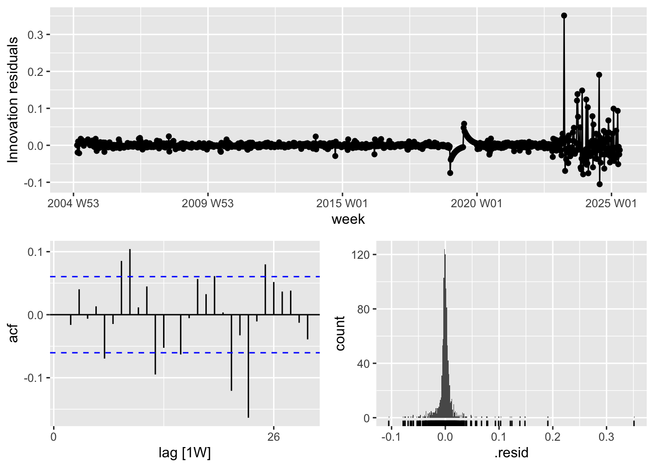
# VAR impulse response
var_irf <- irf(var_fit, impulse = "STAT_ERR",
               response = "RATE", n.ahead = 20)
plot(var_irf)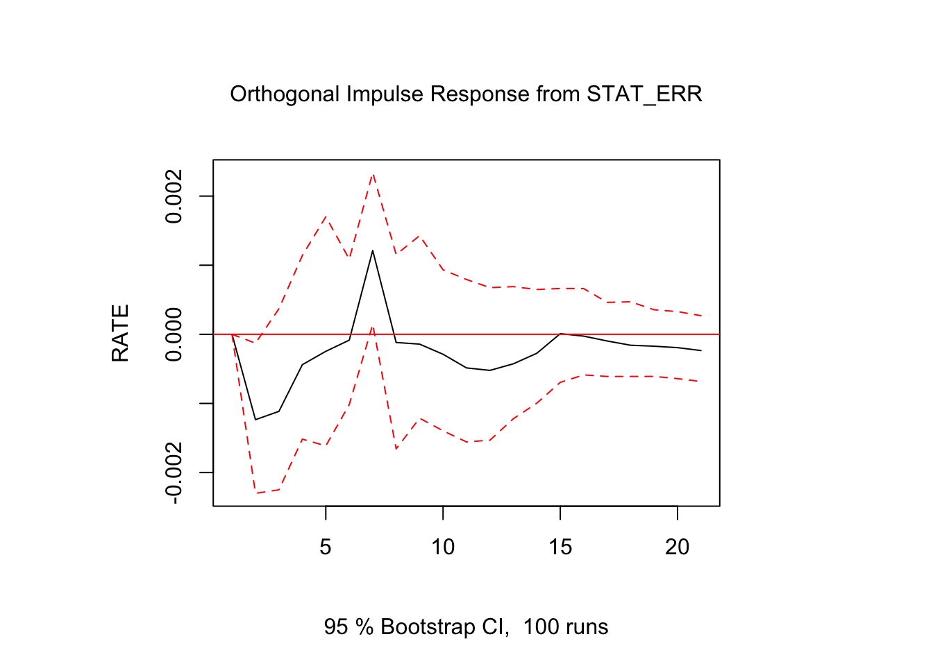
Discussion Questions
Temporal Scaling: The raw data shows ~5,758 daily observations. Why might weekly aggregation improve model performance, and what astrophysical phenomena could be obscured by this smoothing?
Exogenous Variables: For ARIMAX modeling, which additional variables from the dataset would you consider as meaningful predictors of flux (RATE), and how would you test their significance?
VAR Interpretation: If the VAR model shows STAT_ERR Granger-causes RATE but not vice versa, what would this imply about the Swift/BAT instrument’s measurement stability?
Astrophysical vs. Statistical Significance: How might you reconcile a statistically significant ARIMA coefficient (e.g., \(\phi_1 = 0.4274\), \(se = 0.0232\)) with the known physical stability of the Crab Nebula?
Model Selection Tradeoffs: Given the Crab’s role as a calibration source, which model (ETS/ARIMA/VAR) would you recommend for operational forecasting of instrument performance, considering both accuracy and interpretability?