# Retrieve COVID-19 data for the United States and prepare a tsibble
covid_raw <- covid19(country = "US", level = 1, verbose = FALSE) %>%
  as_tsibble(index = date) %>%
  select(date, confirmed, deaths, people_vaccinated) %>%
rename(vaccines = people_vaccinated)Activity43
VAR Modeling and Forecast
We first convert raw cumulative COVID-19 data to new weekly cases/vaccinations using lagged differences. Log-transformation stabilizes variance while preserving relative changes. Weekly aggregation reduces daily reporting noise (e.g., weekend under-reporting).
# Convert to NEW weekly cases
covid_weekly <- covid_raw %>%
  mutate(across(c(confirmed, deaths, vaccines), ~. - lag(.))) %>%
  index_by(week = yearweek(date)) %>%
  summarize(
    cases = sum(confirmed, na.rm = TRUE),
    deaths = sum(deaths, na.rm = TRUE),
    vaccines = sum(vaccines, na.rm = TRUE)
  ) %>%
  filter(cases > 0, deaths > 0, vaccines >= 0) %>%
  mutate(across(c(cases, deaths, vaccines), ~ log(. + 1)))
Activity 1: VAR Modeling - Multivariate Dynamics
VAR System Equations
For variables \(y_1 =\) cases, \(y_2 =\) deaths, \(y_3 =\) vaccines:
\[ \begin{aligned} \Delta \ln(y_{1t}) &= \alpha_1 + \sum_{i=1}^p \phi_{1i} \Delta \ln(y_{1,t-i}) + \sum_{i=1}^p \psi_{1i} \Delta \ln(y_{2,t-i}) + \sum_{i=1}^p \omega_{1i} \Delta \ln(y_{3,t-i}) + \epsilon_{1t} \\ \Delta \ln(y_{2t}) &= \alpha_2 + \sum_{i=1}^p \phi_{2i} \Delta \ln(y_{1,t-i}) + \sum_{i=1}^p \psi_{2i} \Delta \ln(y_{2,t-i}) + \sum_{i=1}^p \omega_{2i} \Delta \ln(y_{3,t-i}) + \epsilon_{2t} \\ \Delta \ln(y_{3t}) &= \alpha_3 + \sum_{i=1}^p \phi_{3i} \Delta \ln(y_{1,t-i}) + \sum_{i=1}^p \psi_{3i} \Delta \ln(y_{2,t-i}) + \sum_{i=1}^p \omega_{3i} \Delta \ln(y_{3,t-i}) + \epsilon_{3t} \end{aligned} \]
Stationarity Diagnostics:
- Individual Stationarity:
# Unit root tests for each series
adf.test(covid_weekly$cases)
    Augmented Dickey-Fuller Test

data:  covid_weekly$cases
Dickey-Fuller = -2.8621, Lag order = 5, p-value = 0.2168
alternative hypothesis: stationaryadf.test(covid_weekly$deaths)
    Augmented Dickey-Fuller Test

data:  covid_weekly$deaths
Dickey-Fuller = -3.0976, Lag order = 5, p-value = 0.1185
alternative hypothesis: stationaryadf.test(covid_weekly$vaccines)
    Augmented Dickey-Fuller Test

data:  covid_weekly$vaccines
Dickey-Fuller = -1.5446, Lag order = 5, p-value = 0.7663
alternative hypothesis: stationary
Activity 2: VAR Modeling
library(vars)

var_data <- covid_weekly %>% as_tibble() %>%
  mutate(across(c(cases, deaths, vaccines), difference)) %>%
  drop_na() %>%
  select(cases, deaths, vaccines)

VARselect(var_data, lag.max=10) # Select lag via IC
$selection
AIC(n) HQ(n) SC(n) FPE(n)
5 2 2 5
$criteria
1 2 3 4 5
AIC(n) -5.018953756 -5.237494422 -5.234885784 -5.235827007 -5.247110180
HQ(n) -4.921103722 -5.066256863 -4.990260699 -4.917814397 -4.855710044
SC(n) -4.778102932 -4.816005481 -4.632758725 -4.453061831 -4.283706885
FPE(n) 0.006611691 0.005314635 0.005330599 0.005329386 0.005275582
6 7 8 9 10
AIC(n) -5.177852792 -5.140110688 -5.044825475 -4.969377318 -4.879798852
HQ(n) -4.713065130 -4.601935501 -4.433262763 -4.284427080 -4.121461089
SC(n) -4.033811380 -3.815431158 -3.539507828 -3.283421553 -3.013204969
FPE(n) 0.005663299 0.005894603 0.006503539 0.007040403 0.007737488var_model <- VAR(var_data, p=5)
serial_test <- serial.test(var_model, lags.pt = 12, type = "PT.adjusted")
serial_test
    Portmanteau Test (adjusted)

data:  Residuals of VAR object var_model
Chi-squared = 41.839, df = 63, p-value = 0.9817
There’s no evidence of leftover serial correlation in the VAR residuals up to 12 lags.
Impulse Response Analysis:
# Impulse Response Analysis
irf(var_model, impulse = "cases", runs = 500, ortho = FALSE, n.ahead = 20) %>% plot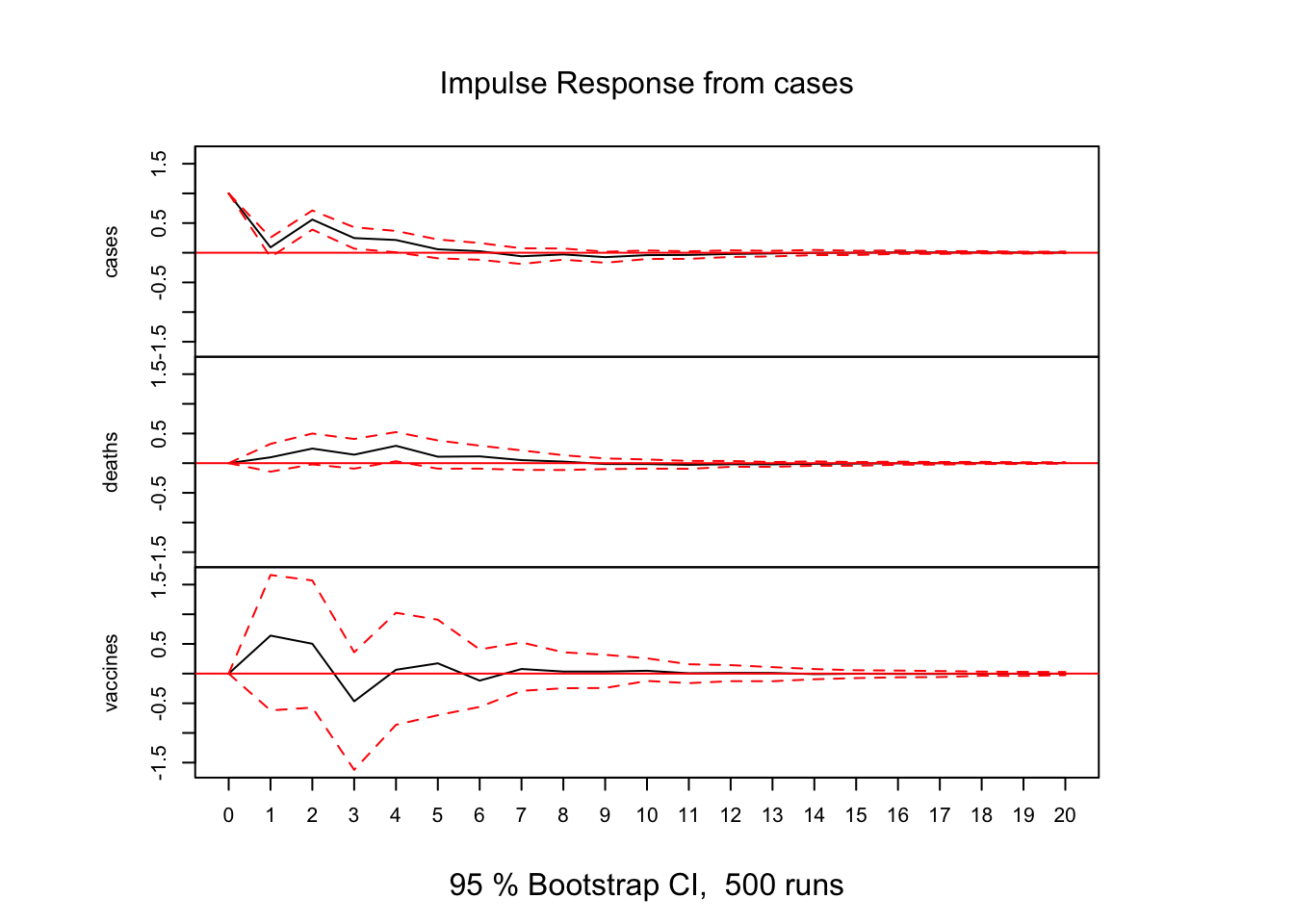
# Impulse Response Analysis
irf(var_model, impulse = "vaccines", runs = 500, ortho = FALSE, n.ahead = 20) %>% plot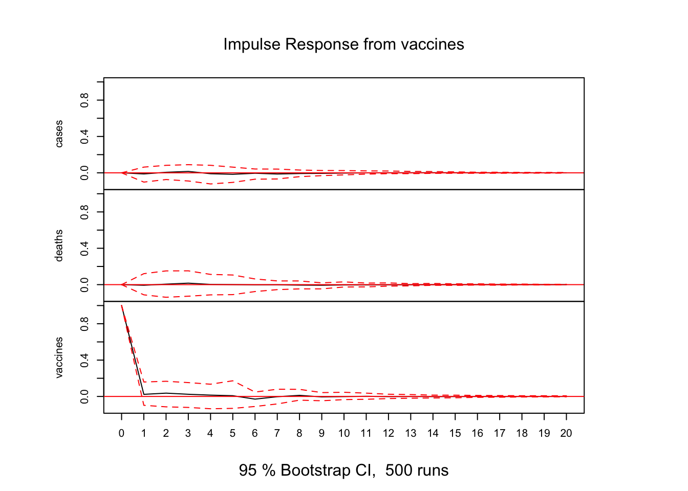
Forecast
A 80/20 train-test split reveals forecast accuracy degradation with longer horizons.
# Train‐test split
n  <- nrow(var_data)
h  <- round(0.2 * n)
train_data <- var_data[1:(n - h), ]
test_data  <- var_data[(n - h + 1):n, ]

# Re‐fit VAR on training
var_train <- VAR(train_data, p = 5)

# Forecast differences for h steps (95% CI)
fcst <- predict(var_train, n.ahead = h, ci = 0.95)

# Extract and back‐transform for "cases"
dif_fcst     <- fcst$fcst$cases[, "fcst"]
last_log     <- tail(covid_weekly$cases[1:(n - h)], 1)
pred_log     <- last_log + cumsum(dif_fcst)
pred_counts  <- exp(pred_log) - 1

# Actual counts in test
actual_log   <- covid_weekly$cases[(n - h + 1):n]
actual_counts<- exp(actual_log) - 1

# Accuracy metrics
library(Metrics)
metrics <- tibble(
  MAE  = mae(actual_counts, pred_counts),
  MAPE = mape(actual_counts, pred_counts),
  RMSE = rmse(actual_counts, pred_counts)
)

# Plot actual vs forecast
plot_df <- tibble(
  week     = covid_weekly$week,
  observed = exp(covid_weekly$cases) - 1
)
test_df <- tibble(
  week     = covid_weekly$week[(n - h + 1):n],
  forecast = pred_counts
)

ggplot(plot_df, aes(week, observed)) +
  geom_line() +
  geom_line(data = test_df, aes(week, forecast), linetype = "dashed") +
  geom_vline(xintercept = as.Date(covid_weekly$week[n - h]), linetype = "dotted") +
  labs(
    title    = "COVID Weekly Cases: Actual vs VAR Forecast",
    subtitle = "Dashed = forecast; dotted line = start of test period",
    x        = "Week", y = "Weekly cases"
  ) +
  theme_minimal()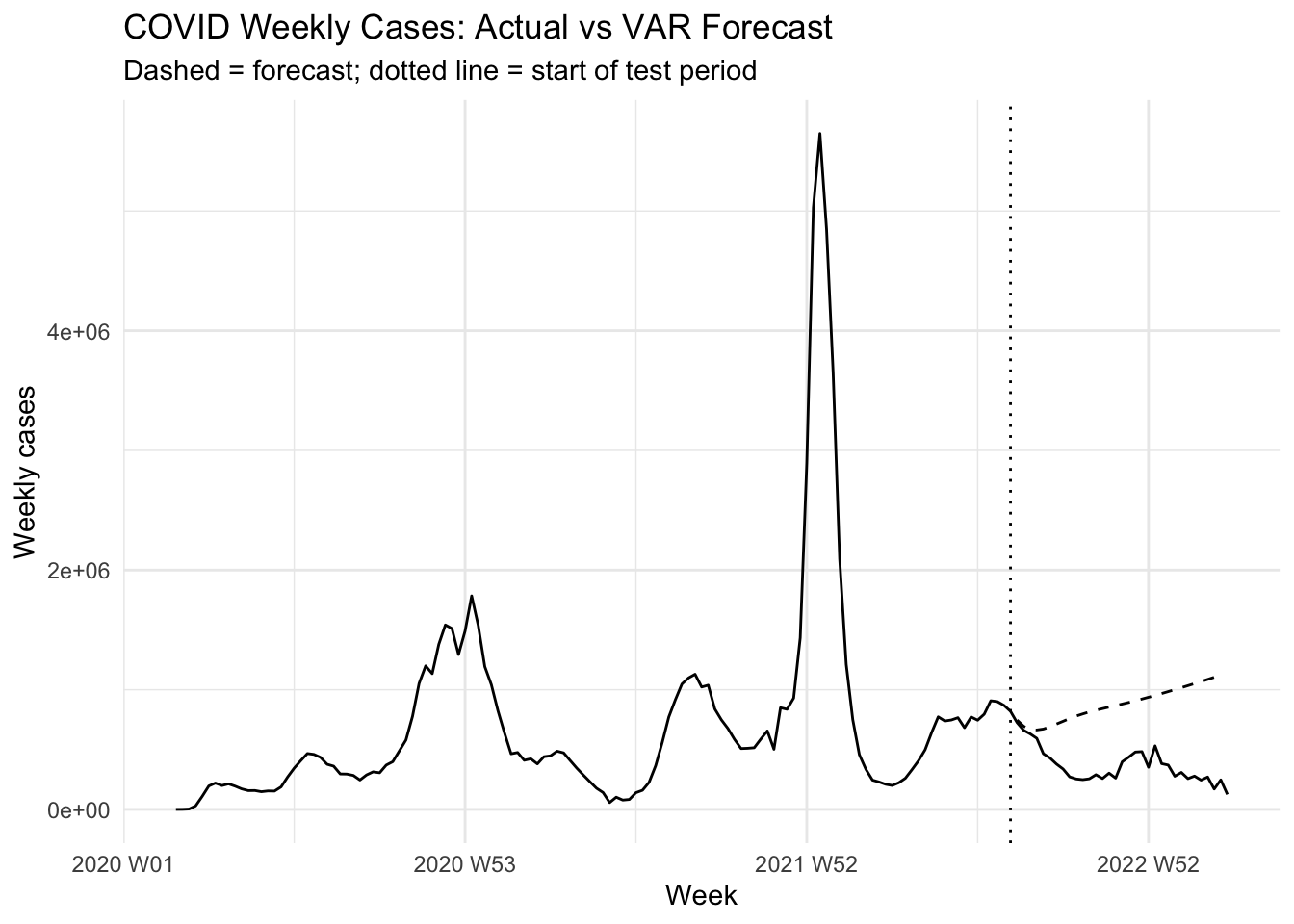
# Show accuracy
metrics
# A tibble: 1 × 3
MAE MAPE RMSE
<dbl> <dbl> <dbl>
1 506499. 1.74 561533.Activity 1: Test–Train Sensitivity
Goal: See how your forecast metrics change if you use a 70/30 split instead of 80/20.
How does a larger test set affect bias and variance in your error estimates?
Plot: Dashed forecast line overlaid on full history, with the split at 70%.
Activity 2: Alternative Variable Set
Goal: Re‑run the pipeline for the pair (deaths, vaccines) only.
Focus: Compare cross‑series dynamics: does a vaccination shock dampen mortality more quickly?
Plot: Two‐series forecast vs. actual, using separate color lines for deaths and vaccines.
Discussion Questions
Split Ratio: What trade‑offs arise when you choose 60/40 vs. 90/10 train/test splits?
Variable Choice: How might including an additional series (e.g. hospitalizations) alter your impulse‑response insights?
Horizon Sensitivity: Why do forecasts typically worsen as lead time increases, and how could you mitigate that?
Evaluation Metrics: When might you prefer MAPE over RMSE (or vice versa) in a public‐health context?