Seasonal Differencing, Rolling Mean, and Rolling Variance
Seasonal Differencing
When a time series exhibits regular, recurring patterns over fixed periods (e.g., 12-month cycles in yearly data), seasonal differencing can help isolate these cyclical components. By subtracting a value from the same season in the previous cycle, you remove much of the repeated seasonal effect:
\[
\text{SeasonalDiff}_t = Y_t - Y_{t-s},
\]
where (s) is the seasonal period (for instance, (s = 12) for monthly data with yearly cycles). This technique is particularly useful for series that show strong periodic fluctuations without requiring other transformations.
Rolling Mean
A rolling mean (or moving average) smooths out short-term fluctuations by averaging consecutive observations within a specified window. For a window size (w), the rolling mean at time (t) is:
This technique helps reveal longer-term trends and cyclical behavior in a time series, since each point is now an average of the most recent (w) observations.
Rolling Variance
A rolling variance measures how dispersed recent values are around their rolling mean within the same window (w). It is calculated as:
Observing the rolling variance over time can highlight periods of increased or decreased fluctuation and help detect heteroscedasticity (changing variance). A more stable rolling variance often indicates that seasonal or cyclic behavior has been accounted for, especially after an appropriate seasonal differencing step.
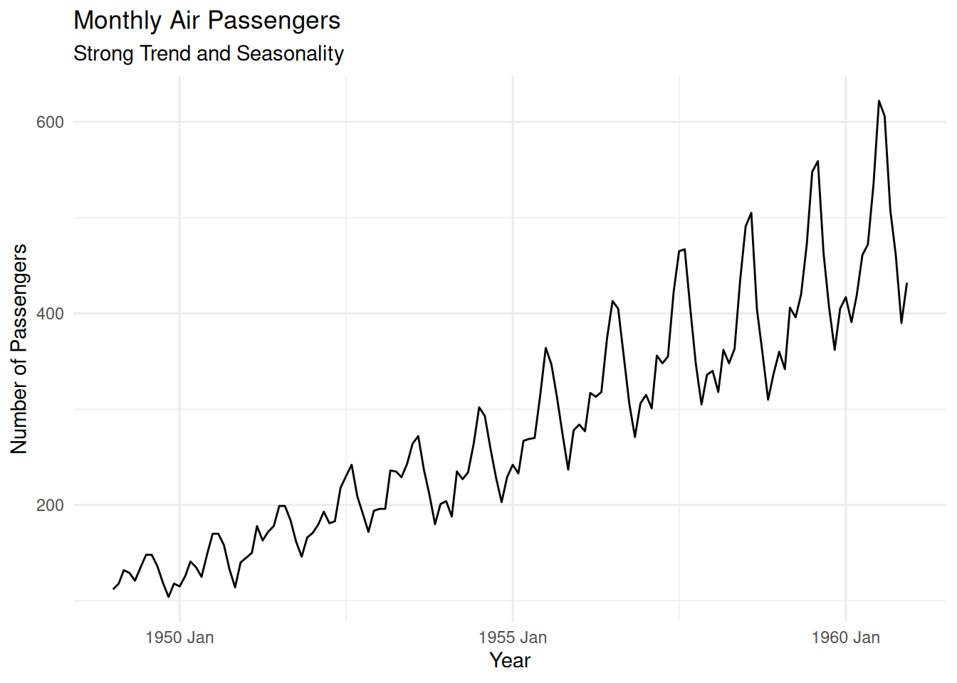
# Convert AirPassengers to a tsibbleairpass <-as_tsibble(AirPassengers) %>%rename(Passengers = value)# Plot the original seriesautoplot(airpass, Passengers) +labs(title ="Monthly Air Passengers", subtitle ="Strong Trend and Seasonality",y ="Number of Passengers", x ="Year") +theme_minimal()
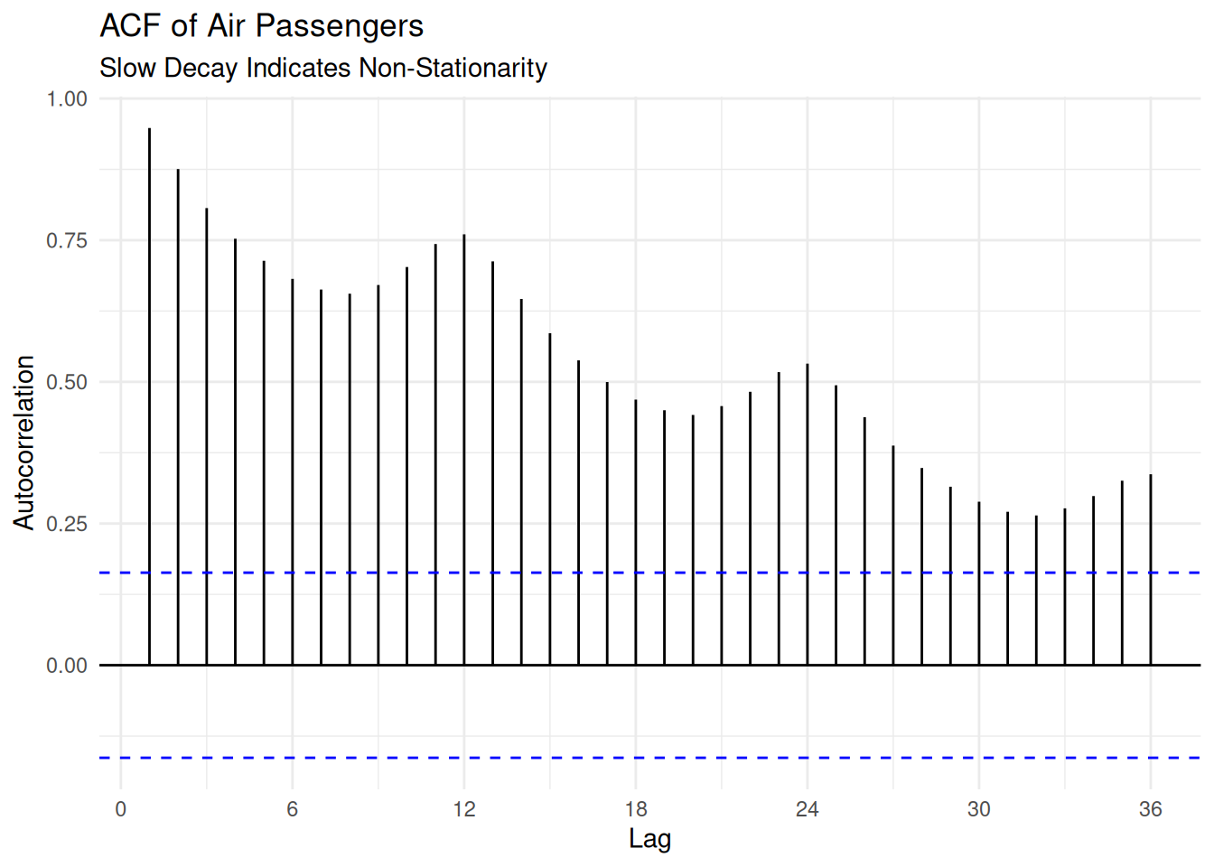
# Compute and plot ACFacf_data <-ACF(airpass, Passengers, lag_max =36)autoplot(acf_data) +labs(title ="ACF of Air Passengers", subtitle ="Slow Decay Indicates Non-Stationarity",y ="Autocorrelation", x ="Lag") +theme_minimal()
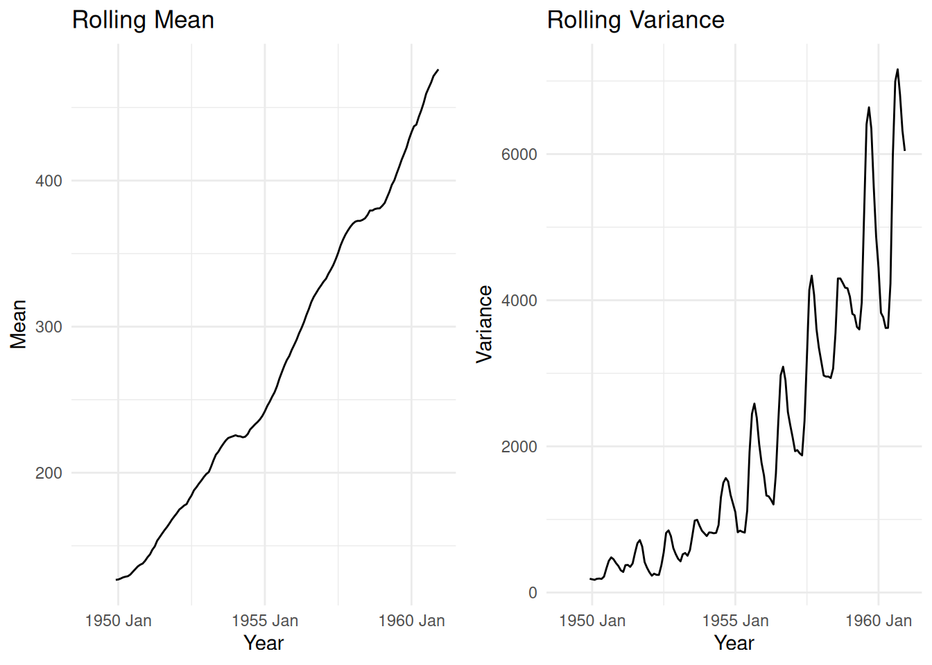
Rolling Statistics
Rolling statistics (mean and variance) help visualize changes in the series over time. For a stationary series, these should remain roughly constant.
Observations:
The rolling mean increases over time, confirming a trend.
The rolling variance also increases, indicating heteroscedasticity.
# Compute rolling mean and varianceairpass_roll <- airpass %>%mutate(RollingMean = slider::slide_dbl(Passengers, mean, .before =11, .complete =TRUE),RollingVar = slider::slide_dbl(Passengers, var, .before =11, .complete =TRUE))# Plot rolling statisticsp_roll <-autoplot(airpass_roll, RollingMean) +labs(title ="Rolling Mean", y ="Mean", x ="Year") +theme_minimal()p_var <-autoplot(airpass_roll, RollingVar) +labs(title ="Rolling Variance", y ="Variance", x ="Year") +theme_minimal()gridExtra::grid.arrange(p_roll, p_var, ncol =2)
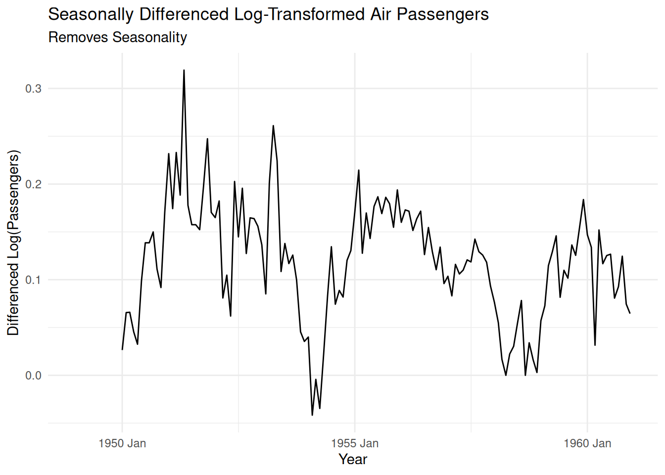
Seasonal Differencing
Seasonal differencing (lag = 12 for monthly data) removes seasonality.
Visualize the Nile dataset to detect any potential seasonality or cyclical components. Even if the Nile data do not exhibit strong seasonal patterns, this initial inspection confirms whether or not seasonal differencing might be warranted.
Compute Rolling Statistics
Rolling Mean: Examine how the mean evolves over a chosen window (e.g., 10 or 12 observations). A stationary series should have a stable rolling mean over time.
Rolling Variance: Similarly, assess how the variance changes (or remains constant) across the same rolling window. Stationarity requires a relatively constant variance.
Seasonal Differencing
If a seasonal pattern is present (e.g., annual cycles in monthly data), remove it by differencing observations separated by one full season. This step is relevant if the data exhibit cyclical or repeating patterns at fixed intervals.
Interpretation
Evaluate how rolling mean and variance behave post-seasonal differencing (if performed).
Verify if stationarity indicators (constant mean, constant variance) are satisfied.
Reflection Questions:
Does the Nile dataset exhibit any trends or seasonality?
How do the rolling statistics (mean and variance) behave over time?
What transformations, if any, are necessary to achieve stationarity?
Investigate any repeating or cyclical behavior in the annual Lynx data that might hint at seasonal or quasi-seasonal effects.
Compute Rolling Statistics
Rolling Mean: Check if the mean stays relatively stable over a certain window, which supports stationarity.
Rolling Variance: Verify whether variance remains relatively constant over time.
Seasonal Differencing
If the Lynx data show cyclical behavior at fixed intervals (e.g., periodic surges), seasonal differencing with an appropriate lag can reduce these cycles to produce a more stationary series.
Interpretation
Compare rolling mean and variance before and after seasonal differencing to confirm stationarity improvements.
Discuss whether the cyclical patterns are effectively removed or diminished.
Reflection Questions
Does the Lynx dataset exhibit any notable trends or cyclic patterns?
How do the rolling mean and variance behave over time?
Are transformations necessary to ensure stationarity?