Activity22

Theoretical Foundations of MA Processes

Time Series Nature & Invertibility

Definition:

MA(\(q\)) model:
\(Y_t = \epsilon_t + \theta_1 \epsilon_{t-1} + \cdots + \theta_q \epsilon_{t-q}\)
where \(\epsilon_t \sim WN(0,\sigma^2)\)

Key Properties:

• Models shock persistence through lagged errors
  
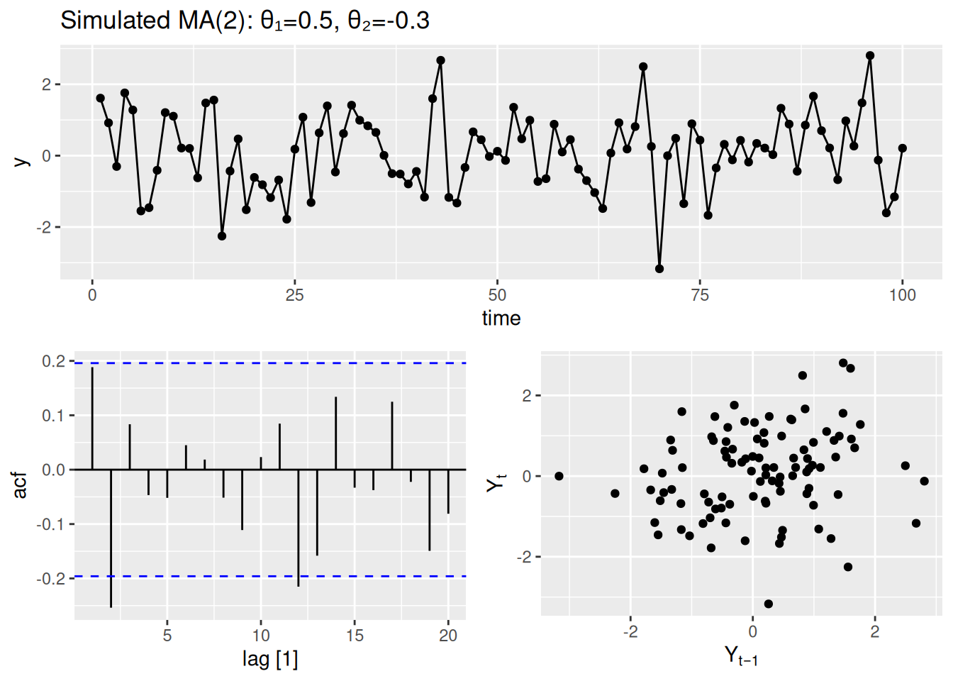
• ACF cuts off after lag \(q\) (distinct signature)
  
• PACF tails off gradually
  
• Requires invertibility (roots of \(1 + \theta_1 z + \cdots + \theta_q z^q = 0\) lie outside unit circle)

---

Simulating & Diagnosing MA Processes

Simulated MA(2) Process

library(fable)
set.seed(123)
ma_data <- tibble(
  time = 1:100,
  y = arima.sim(model = list(ma = c(0.5, -0.3)), n = 100) # θ₁=0.5, θ₂=-0.3
) %>% as_tsibble(index = time)

ma_data %>% 
  gg_tsdisplay(y, plot_type = "scatter") + # Observe ACF cutoff at lag 2
  labs(title = "Simulated MA(2): θ₁=0.5, θ₂=-0.3")

Model Estimation & Diagnostics

fit_ma <- ma_data %>% 
  model(ARIMA(y ~ pdq(0,0,2))) # Explicit MA(2) specification

report(fit_ma) # Check θ estimates vs true values (0.5, -0.3)

Series: y 
Model: ARIMA(0,0,2) 

Coefficients:
         ma1      ma2
      0.5477  -0.3881
s.e.  0.0911   0.0908

sigma^2 estimated as 0.8128:  log likelihood=-131.49
AIC=268.98   AICc=269.23   BIC=276.8

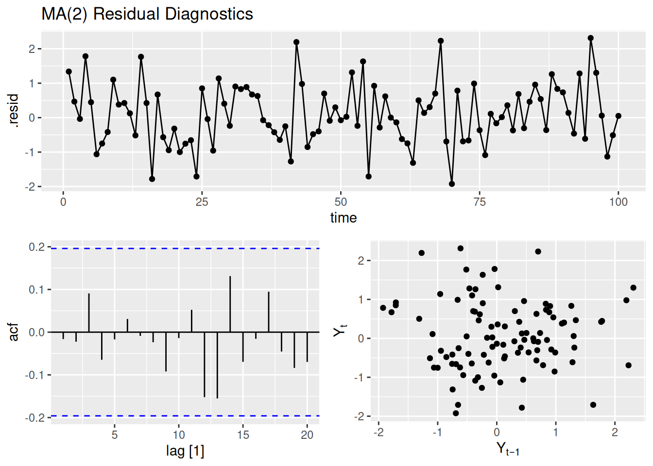
fit_ma %>% 
  residuals() %>% 
  gg_tsdisplay(plot_type = "scatter") + 
  labs(title = "MA(2) Residual Diagnostics")

---

Real-World Case Study: US Consumption

Lab Activity A: Modeling Consumption with MA

1. Data Preparation

2. Exploratory Analysis

3. MA Order Identification

4. Model Fitting

5. Residual Diagnostics

6. Forecasting

---

Lab Activity B: Modeling US Production

1. Data Preparation

2. Visualize Series

3. MA Order Selection

Determine appropriate MA order through ACF:

4. Model Comparison

Fit competing specifications and evaluate:

5. Policy-Relevant Forecasting

Using the best model, generate forecasts up-to 10 time points into the future and interpret economic meaning:

Key Concepts Cheat Sheet

Feature	MA(\(q\))	Contrast with AR(\(p\))
ACF	Cuts off at lag \(q\)	Tails off gradually
PACF	Tails off gradually	Cuts off at lag \(p\)
Condition	Invertibility (roots > 1)	Stationarity (roots < 1)
Use Case	Short-lived shock effects	Long-term dependencies