# Retrieve COVID-19 data for the United States and prepare a tsibble
# Get cumulative COVID metrics
covid_raw <- covid19(country = "US", level = 1, verbose = FALSE) %>%
  as_tsibble(index = date) %>%
  select(date, confirmed, people_vaccinated) %>%
rename(vaccines = people_vaccinated)Activity42
ARCH Effects in Case Volatility
Data Preparation
We first convert raw cumulative COVID-19 data to new weekly cases/vaccinations using lagged differences. Log-transformation stabilizes variance while preserving relative changes. Weekly aggregation reduces daily reporting noise (e.g., weekend under-reporting).
# Convert to NEW weekly cases
covid_weekly <- covid_raw %>%
  mutate(across(c(confirmed, vaccines), ~. - lag(.))) %>% # Calculate daily changes
  index_by(week = yearweek(date)) %>%
  summarize(
    cases = sum(confirmed, na.rm = TRUE),
    vaccines = sum(vaccines, na.rm = TRUE)
  ) %>%
  filter(cases > 0, vaccines >= 0) %>%
  mutate(across(c(cases, vaccines), ~ log(. + 1)))
1. Residual Diagnostics
Activity 1: Residuals Volatility Analysis
library(strucchange)

bp_multi <- breakpoints(cases ~ 1 + vaccines, data = covid_weekly, h = 0.05, breaks = 3)
break_dates <- covid_weekly$week[bp_multi$breakpoints]

# Create intervention dummy
library(fastDummies)
covid_weekly <- covid_weekly %>%
  mutate(
    intervention_period = case_when(
      week < break_dates[1] ~ "pre",
      week >= break_dates[1] & week < break_dates[2] ~ "phase1",
      week >= break_dates[2] & week < break_dates[3] ~ "phase2",
      week >= break_dates[3] ~ "post"
    )
  ) %>%
  dummy_cols(select_columns = "intervention_period")  %>%
  as_tsibble(index = week)

arima_model <- covid_weekly %>%
  model(fable::ARIMA(cases ~ vaccines + intervention_period))

report(arima_model)
Series: cases
Model: LM w/ ARIMA(3,0,2)(1,0,0)[52] errors
Coefficients:
ar1 ar2 ar3 ma1 ma2 sar1 vaccines
2.2057 -1.6628 0.4427 -0.9343 0.7572 0.0876 0.0007
s.e. 0.1185 0.2460 0.1407 0.0887 0.0845 0.1161 0.0152
intervention_periodphase2 intervention_periodpost
0.062 0.2065
s.e. 0.235 0.3108
intervention_periodpre intercept
-0.2380 11.5382
s.e. 0.2447 1.4644
sigma^2 estimated as 0.08206: log likelihood=-25.9
AIC=75.79 AICc=77.83 BIC=113.14arima_model %>%
residuals() %>%
ggplot(aes(x = week, y = .resid)) +
geom_line() + geom_point() +
labs(title = "COVID Case Model Residuals")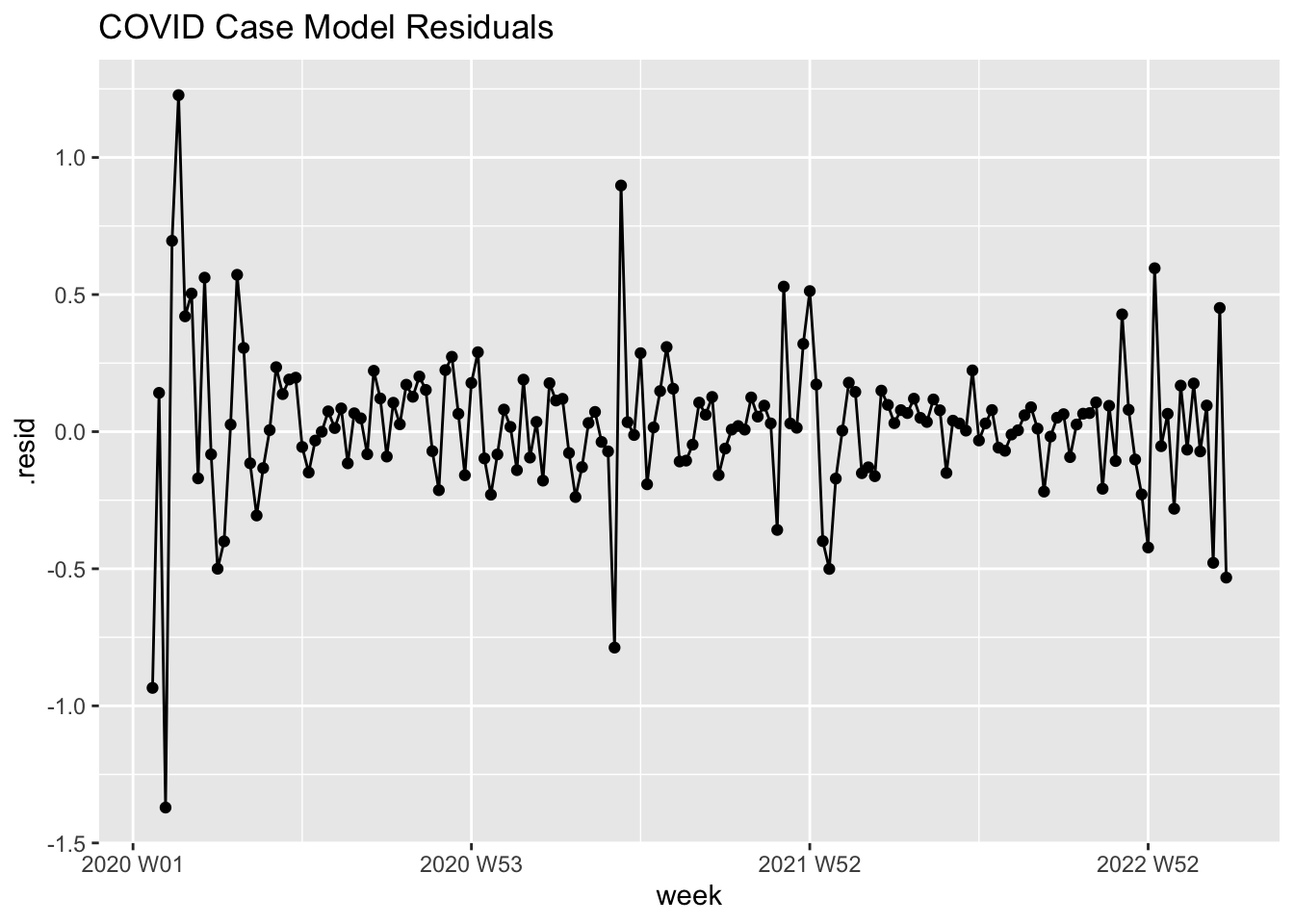
Graphical Analysis
First, let’s examine residuals from our intervention ARIMA model visually:
squared_residual_plot <- arima_model %>%
  residuals() %>%
  mutate(sq_resid = .resid^2) %>%
  ggplot(aes(x = week, y = sq_resid)) +
  geom_line() + geom_point() +
  labs(title = "Squared Residuals Highlight ARCH Effects",
       subtitle = "Persistent variance changes indicate volatility clustering")

squared_residual_plot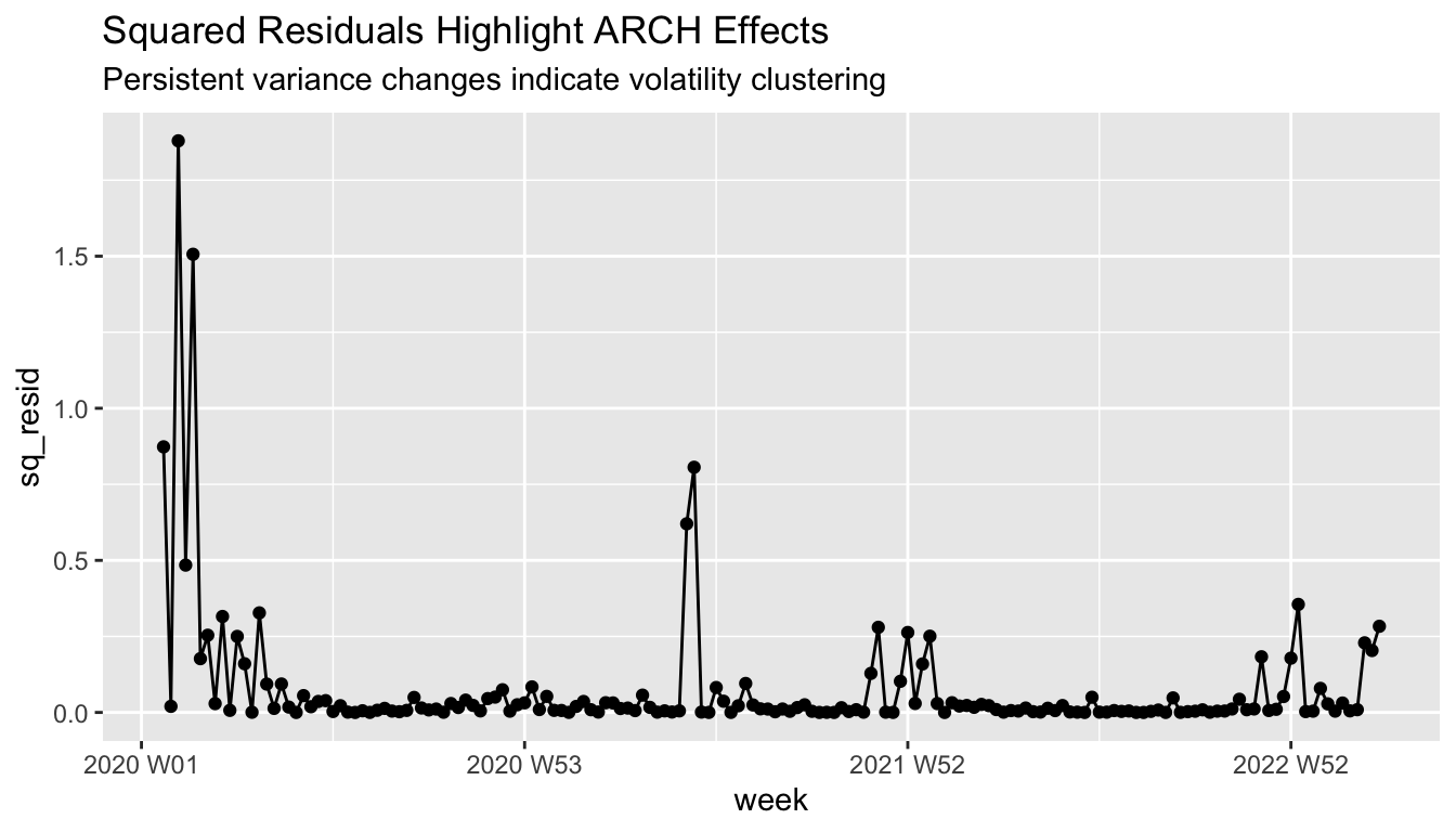
- Residuals show clear volatility clustering (periods of high/low dispersion)
- Squared residuals demonstrate time-varying variance - violates constant variance assumption
Activity 2: ARCH LM Test
library(FinTS)
residuals <- resid(arima_model) %>% pull(.resid)
ArchTest(residuals, lags = 4)
    ARCH LM-test; Null hypothesis: no ARCH effects

data:  residuals
Chi-squared = 64.113, df = 4, p-value = 3.957e-13
The significant p-value (<<0.05) rejects the null hypothesis of no ARCH effects, confirming volatility clustering needs modeling.
3. GARCH Modeling
Model Specification
We use GARCH(1,1) to model both:
- ARCH term (\(\alpha\)): Immediate shock impact
- GARCH term (\(\beta\)): Persistent volatility memory
# GARCH(1,1) Estimation
library(rugarch)

# Use ARIMA residuals as input series
garch_spec <- ugarchspec(
  variance.model = list(model = "sGARCH", garchOrder = c(1,1)),
  mean.model = list(armaOrder = c(3,0), include.mean = FALSE)
)

garch_fit <- ugarchfit(
  spec = garch_spec,
  data = residuals[!is.na(residuals)] # Remove NA from differencing
)

garch_fit
*---------------------------------*
*          GARCH Model Fit        *
*---------------------------------*

Conditional Variance Dynamics
-----------------------------------
GARCH Model : sGARCH(1,1)
Mean Model  : ARFIMA(3,0,0)
Distribution    : norm

Optimal Parameters
------------------------------------
        Estimate  Std. Error  t value Pr(>|t|)
ar1     0.042417    0.111648  0.37992 0.704009
ar2    -0.053242    0.101358 -0.52529 0.599385
ar3    -0.363783    0.110194 -3.30130 0.000962
omega   0.010593    0.002734  3.87514 0.000107
alpha1  0.342966    0.115412  2.97168 0.002962
beta1   0.422297    0.102669  4.11318 0.000039

Robust Standard Errors:
        Estimate  Std. Error  t value Pr(>|t|)
ar1     0.042417    0.183638  0.23098 0.817331
ar2    -0.053242    0.134968 -0.39448 0.693229
ar3    -0.363783    0.190919 -1.90543 0.056724
omega   0.010593    0.004455  2.37767 0.017422
alpha1  0.342966    0.084932  4.03813 0.000054
beta1   0.422297    0.082181  5.13860 0.000000

LogLikelihood : 18.8111

Information Criteria
------------------------------------

Akaike       -0.154351
Bayes        -0.041869
Shibata      -0.156844
Hannan-Quinn -0.108694

Weighted Ljung-Box Test on Standardized Residuals
------------------------------------
                         statistic  p-value
Lag[1]                       3.200 0.073660
Lag[2*(p+q)+(p+q)-1][8]      6.256 0.004592
Lag[4*(p+q)+(p+q)-1][14]     7.285 0.504281
d.o.f=3
H0 : No serial correlation

Weighted Ljung-Box Test on Standardized Squared Residuals
------------------------------------
                        statistic p-value
Lag[1]                      0.124  0.7247
Lag[2*(p+q)+(p+q)-1][5]     4.214  0.2285
Lag[4*(p+q)+(p+q)-1][9]     5.268  0.3911
d.o.f=2

Weighted ARCH LM Tests
------------------------------------
            Statistic Shape Scale P-Value
ARCH Lag[3]    0.1476 0.500 2.000  0.7008
ARCH Lag[5]    1.5388 1.440 1.667  0.5822
ARCH Lag[7]    1.8114 2.315 1.543  0.7572

Nyblom stability test
------------------------------------
Joint Statistic:  1.448
Individual Statistics:
ar1    0.74404
ar2    0.12425
ar3    0.16236
omega  0.06102
alpha1 0.05590
beta1  0.04914

Asymptotic Critical Values (10% 5% 1%)
Joint Statistic:         1.49 1.68 2.12
Individual Statistic:    0.35 0.47 0.75

Sign Bias Test
------------------------------------
                   t-value   prob sig
Sign Bias           0.4036 0.6870
Negative Sign Bias  0.1300 0.8967
Positive Sign Bias  0.2986 0.7657
Joint Effect        0.6799 0.8779


Adjusted Pearson Goodness-of-Fit Test:
------------------------------------
  group statistic p-value(g-1)
1    20     25.81      0.13565
2    30     48.34      0.01356
3    40     56.65      0.03355
4    50     70.75      0.02266


Elapsed time : 0.03699303
Model Equation
\[ \sigma_t^2 = 0.0106 + 0.343\epsilon_{t-1}^2 + 0.422\sigma_{t-1}^2 \]
Key Updates: 1. Persistence: \(\alpha + \beta = 0.343 + 0.422 = 0.765\)
2. Half-life: \(\log(0.5)/\log(0.765) \approx 2.58\) weeks
Model Diagnostics
library(ggfortify)
std_resid <- residuals(garch_fit, standardize=TRUE)

dat <- fortify.zoo(std_resid)

# Now create the Q-Q plot using the converted data
ggplot(dat, aes(sample = std_resid)) +
  stat_qq() +
  geom_abline(slope = 1, intercept = 0, color = "red")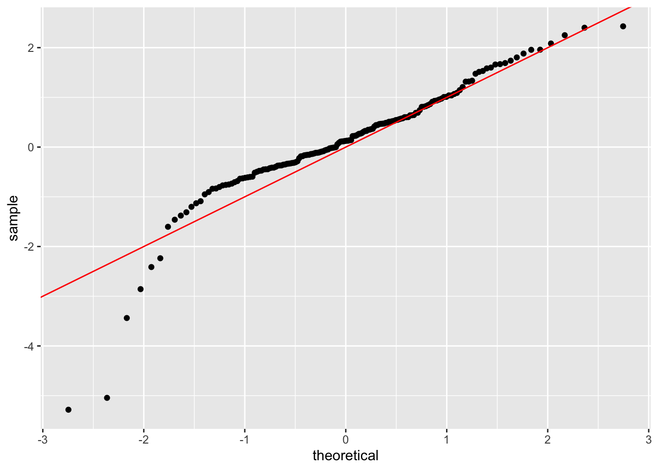
Diagnostic Checks:
- No significant autocorrelation in squared residuals → GARCH captures volatility clustering
- QQ-plot shows heavier tails than normal distribution → Consider Student-t innovations
4. Forecasting with GARCH
Conditional Variance Forecast
garch_forecast <- ugarchforecast(garch_fit, n.ahead = 20)
plot(garch_forecast, which = 3)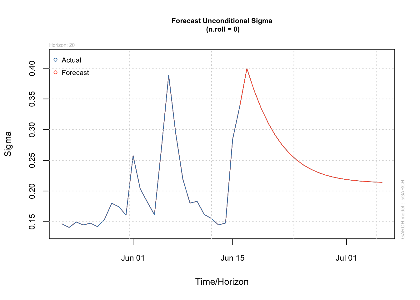
Forecast Interpretation: - Volatility slowly mean-reverts due to high persistence - Prediction intervals widen initially then stabilize
5. Asymmetric Volatility with EGARCH
Model Implementation
egarch_spec <- ugarchspec(
  variance.model = list(model = "eGARCH"),
  mean.model = list(armaOrder = c(3,0), include.mean = FALSE)
)

egarch_fit <- ugarchfit(egarch_spec, data = residuals[!is.na(residuals)])

egarch_fit
*---------------------------------*
*          GARCH Model Fit        *
*---------------------------------*

Conditional Variance Dynamics
-----------------------------------
GARCH Model : eGARCH(1,1)
Mean Model  : ARFIMA(3,0,0)
Distribution    : norm

Optimal Parameters
------------------------------------
        Estimate  Std. Error  t value Pr(>|t|)
ar1      0.18186    0.103358   1.7596 0.078483
ar2     -0.13284    0.086495  -1.5358 0.124576
ar3     -0.34822    0.096555  -3.6065 0.000310
omega   -0.49365    0.158187  -3.1206 0.001805
alpha1  -0.32572    0.084450  -3.8570 0.000115
beta1    0.83480    0.046362  18.0061 0.000000
gamma1   0.46821    0.110173   4.2497 0.000021

Robust Standard Errors:
        Estimate  Std. Error  t value Pr(>|t|)
ar1      0.18186    0.152147   1.1953 0.231965
ar2     -0.13284    0.095333  -1.3935 0.163482
ar3     -0.34822    0.131049  -2.6572 0.007879
omega   -0.49365    0.205857  -2.3980 0.016485
alpha1  -0.32572    0.114213  -2.8519 0.004346
beta1    0.83480    0.056665  14.7323 0.000000
gamma1   0.46821    0.136197   3.4377 0.000587

LogLikelihood : 23.93619

Information Criteria
------------------------------------

Akaike       -0.204050
Bayes        -0.072822
Shibata      -0.207419
Hannan-Quinn -0.150784

Weighted Ljung-Box Test on Standardized Residuals
------------------------------------
                         statistic p-value
Lag[1]                       2.620 0.10550
Lag[2*(p+q)+(p+q)-1][8]      5.691 0.03285
Lag[4*(p+q)+(p+q)-1][14]     6.655 0.62830
d.o.f=3
H0 : No serial correlation

Weighted Ljung-Box Test on Standardized Squared Residuals
------------------------------------
                        statistic p-value
Lag[1]                    0.03506  0.8515
Lag[2*(p+q)+(p+q)-1][5]   4.43440  0.2046
Lag[4*(p+q)+(p+q)-1][9]   5.96715  0.3020
d.o.f=2

Weighted ARCH LM Tests
------------------------------------
            Statistic Shape Scale P-Value
ARCH Lag[3]    0.4855 0.500 2.000  0.4860
ARCH Lag[5]    1.1793 1.440 1.667  0.6806
ARCH Lag[7]    1.9199 2.315 1.543  0.7343

Nyblom stability test
------------------------------------
Joint Statistic:  1.5439
Individual Statistics:
ar1    0.84216
ar2    0.10204
ar3    0.06074
omega  0.03966
alpha1 0.06067
beta1  0.04564
gamma1 0.05945

Asymptotic Critical Values (10% 5% 1%)
Joint Statistic:         1.69 1.9 2.35
Individual Statistic:    0.35 0.47 0.75

Sign Bias Test
------------------------------------
                   t-value   prob sig
Sign Bias          0.09363 0.9255
Negative Sign Bias 0.50412 0.6149
Positive Sign Bias 0.15848 0.8743
Joint Effect       0.28269 0.9633


Adjusted Pearson Goodness-of-Fit Test:
------------------------------------
  group statistic p-value(g-1)
1    20     24.12       0.1916
2    30     29.90       0.4188
3    40     34.00       0.6970
4    50     50.87       0.3999


Elapsed time : 0.03595304
EGARCH Equation
\[ \begin{aligned} \ln(\sigma_t^2) &= -0.493 + 0.835\ln(\sigma_{t-1}^2) + \\ &\quad 0.468\left(\frac{|\epsilon_{t-1}|}{\sigma_{t-1}} - \sqrt{2/\pi}\right) - 0.326\frac{\epsilon_{t-1}}{\sigma_{t-1}} \end{aligned} \]
Key Parameters: - \(\gamma = 0.468\) (positive asymmetric effect) - Negative \(\alpha = -0.326\) confirms leverage effect (negative shocks increase volatility more than positive ones)
Q1: Why does the ARCH(1) coefficient (\(\alpha=0.343\)) in pre-vaccine residuals suggest public health volatility?
Q2: The GARCH(1,1) persistence (\(\alpha+\beta=0.765\)) remains high post-vaccine. What does this mean for forecasting?
Q3: Why does the log transformation of cases (+1) make sense for volatility modeling, and what would happen if we used raw case counts?
Q4: The QQ-plot shows heavier tails than normal distribution. How does this impact our interpretation of “extreme case surge” probabilities?
Q5: The volatility half-life is ~2.58 weeks. What real-world public health processes might explain this persistence?