# Load data
<- read_csv("~/Desktop/Math493Spring25ClassMaterials/data/google.csv")
google <- google |>
google_stock as_tsibble() |>
mutate(LogClose = log(Close)) # Log-transform for later use
# Plot original series
|>
google_stock autoplot(Close) +
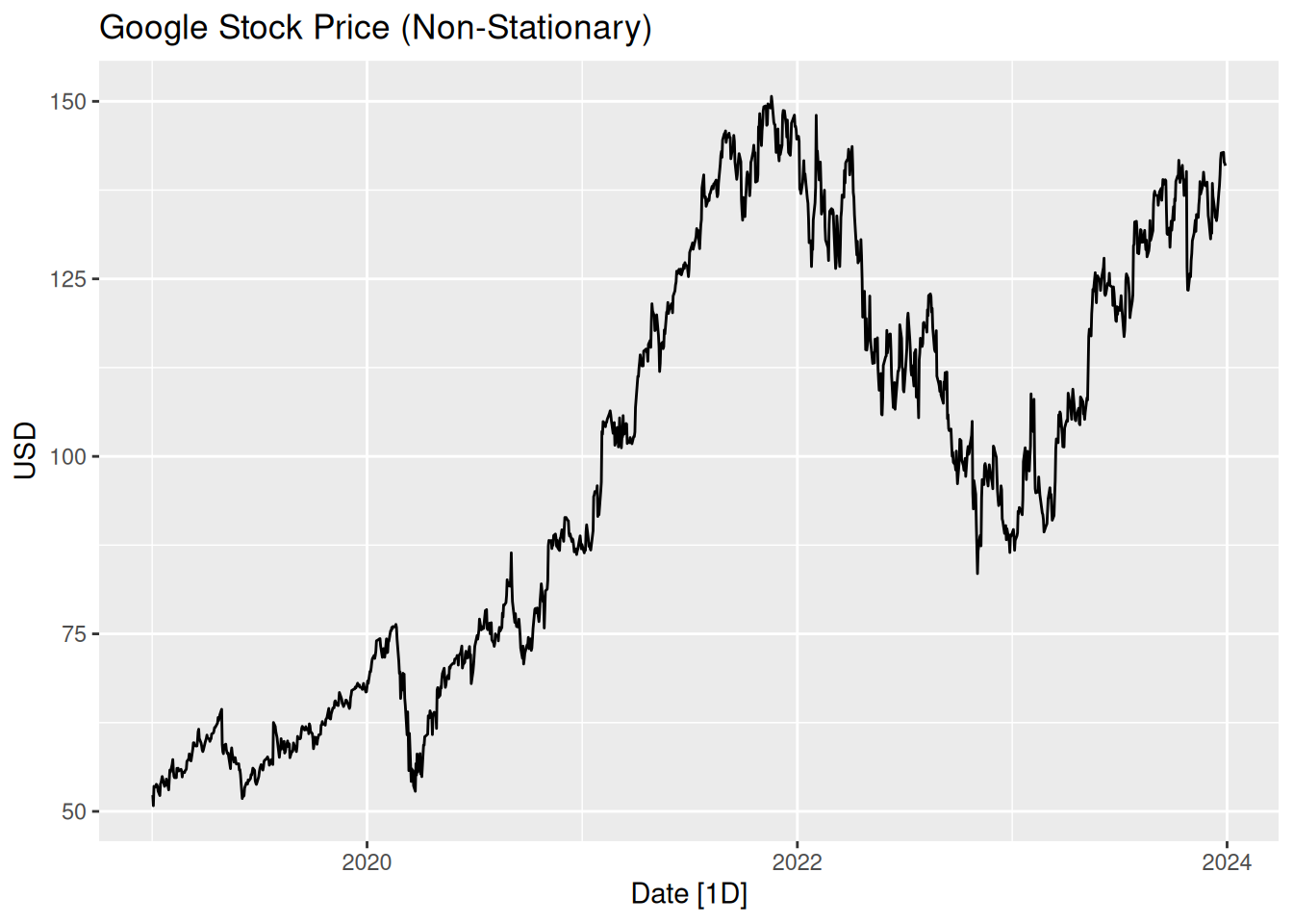
labs(title = "Google Stock Price (Non-Stationary)", y = "USD")
Activity5
Differencing, Transformations, and Stationarity
What is Stationarity?
A time series is stationary if its statistical properties (mean, variance, autocorrelation) do not change over time. Stationarity is a key assumption for many time series models (e.g., ARIMA). Non-stationary series often exhibit:
- Trends: A long-term increase or decrease in the data.
- Seasonality: Periodic fluctuations.
- Changing Variance: Variability that increases or decreases over time.
Transformations to Achieve Stationarity
- Differencing: Removes trends by computing the difference between consecutive observations.
- Formula: \(\nabla X_t = X_t - X_{t-1}\)
- Log Transformation: Stabilizes multiplicative variance by applying the natural logarithm.
- Formula: \(Y_t = \log(X_t)\)
- Box-Cox Transformation: A generalized power transformation that stabilizes variance and can handle non-linear trends.
- Formula: \(Y_t = \frac{X_t^\lambda - 1}{\lambda}\)
Step 1: Visualize Non-Stationary Data
We start by loading and visualizing a non-stationary time series (Google stock prices).
Observation: The upward trend indicates non-stationarity.
Step 2: Statistical Tests for Stationarity
Use the KPSS test (null hypothesis: stationarity) and ADF test (null hypothesis: unit root) to confirm non-stationarity.
# KPSS test
|>
google_stock features(Close, unitroot_kpss)
# A tibble: 1 × 2
kpss_stat kpss_pvalue
<dbl> <dbl>
1 10.6 0.01
# Suggested differencing order
|>
google_stock features(Close, unitroot_ndiffs)
# A tibble: 1 × 1
ndiffs
<int>
1 1
Interpretation:
KPSS p-value < 0.05 ⇒ Reject stationarity.
unitroot_ndiffs
suggests the number of differences required (e.g., 1).
Step 3: Apply Differencing
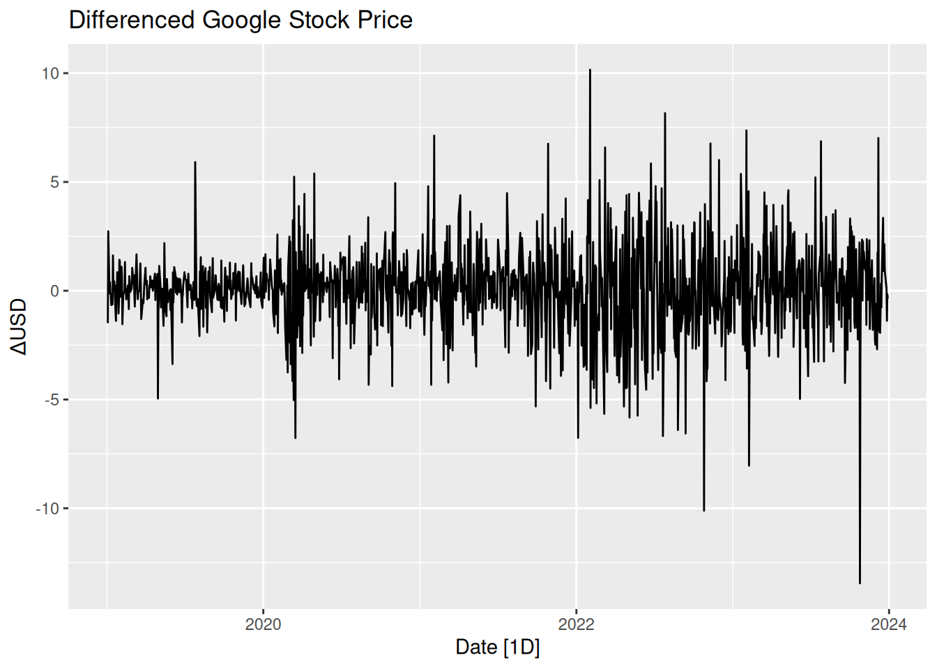
Differencing removes trends by computing the difference between consecutive observations.
# First difference
<- google_stock |>
google_stationary mutate(DiffClose = difference(Close))
# Plot differenced series
|>
google_stationary autoplot(DiffClose) +
labs(title = "Differenced Google Stock Price", y = "ΔUSD")
Observation: The differenced series has a stabilized mean.
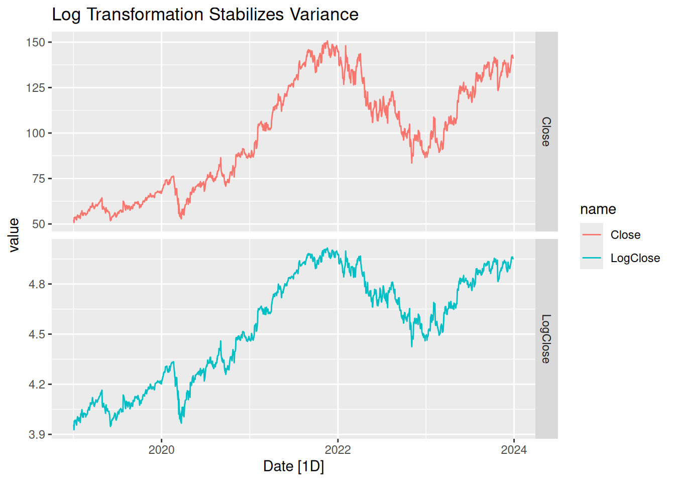
Step 4: Apply Log Transformation
Log transformations stabilize multiplicative variance.
# Plot original vs log-transformed series
|>
google_stock pivot_longer(c(Close, LogClose)) |>
autoplot(value) +
facet_grid(name ~ ., scales = "free_y") +
labs(title = "Log Transformation Stabilizes Variance")
Observation: The log-transformed series shows reduced variance amplification.
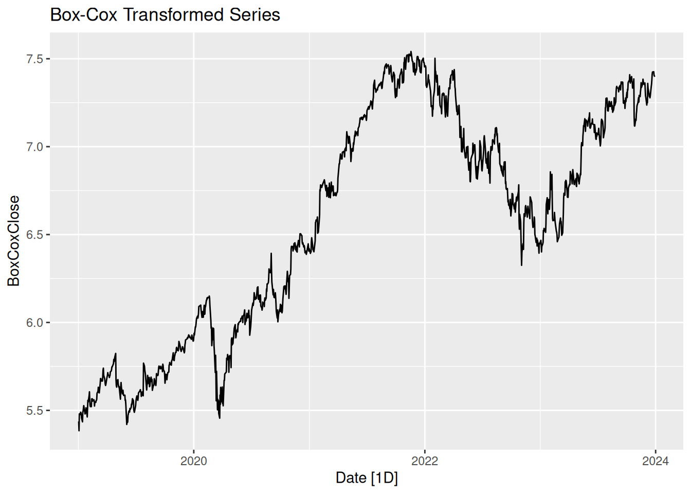
Step 5: Apply Box-Cox Transformation
The Box-Cox transformation generalizes log and power transformations.
# Estimate optimal lambda
<- google_stock |>
lambda features(Close, features = guerrero) |>
pull(lambda_guerrero)
# Apply Box-Cox transformation
|>
google_stock mutate(BoxCoxClose = box_cox(Close, lambda)) |>
autoplot(BoxCoxClose) +
labs(title = "Box-Cox Transformed Series")
Observation: The Box-Cox transformation stabilizes both mean and variance.
Lab Activity
Prompt 1: Load and Visualize Data
- Load the
global_economy
dataset from thetsibble
package. - Plot GDP for a specific country (e.g., “United States”). Assess stationarity visually.
Solution:
Prompt 2: Test for Stationarity
- Use the KPSS test to check for stationarity.
- Determine the required differencing order using
unitroot_ndiffs
.
Solution:
Prompt 3: Apply Transformations
- Apply first differencing to the GDP series.
- Apply a Box-Cox transformation using Guerrero’s method to estimate λ.
- Re-test stationarity using the KPSS test.
Solution: