# Prepare data & dummy
us_change <- us_change %>%
mutate(gfc = Quarter >= yearquarter("2008 Q3"))Activity52
Distributional Drift (us_change)
Ethical Consideration: Detecting structural breaks from historical events
🎯 Intervention in Time Series Models
- Clearly define intervention point
- Compare “with” vs. “without” intervention in a single
model()call
- Maintain consistent train/test split for fair evaluation ✅
- Compute out-of-sample accuracy (RMSE, MAE) on identical horizons 📈
h <- 8  # forecast horizon in quarters
train <- us_change %>%
  slice(1:(n() - h))
test  <- us_change %>%
  slice_tail(n = h)
models <- train %>%
mutate(gfc = Quarter >= yearquarter("2008 Q3")) %>%
model(
with_gfc = ARIMA(Unemployment ~ gfc),
no_gfc = ARIMA(Unemployment ~ 1)
)fc <- forecast(models, new_data = test)
# Compute Out-of-Sample Accuracy
acc <- accuracy(fc, test)
acc %>% select(.model, RMSE, MAE) %>%
knitr::kable(caption = "Forecast Accuracy Metrics")| .model | RMSE | MAE |
|---|---|---|
| no_gfc | 0.177429 | 0.1546663 |
| with_gfc | 0.134225 | 0.1104528 |
# Comparison Plot
autoplot(train, Unemployment) +
  autolayer(test, Unemployment, linetype = "dashed") +
  autolayer(fc, aes(.mean, colour = .model), size = 1.1) +
  scale_colour_manual(
    values = c(with_gfc = "steelblue", no_gfc = "firebrick") ) +   theme(
    legend.position = "none") +
  coord_cartesian(xlim = yearquarter(c("2008 Q1", "2020 Q1"))) +
  labs(
    title    = "US Unemployment: Actual vs. Forecasts",
    subtitle = "Solid = train; Dashed = test; Blue/Red = forecasts (with/without GFC)",
    x = NULL, y = "Unemployment (%)"
  ) +
  theme_minimal() +
  theme(
    legend.position = "bottom",
    strip.text       = element_text(face = "bold")
  )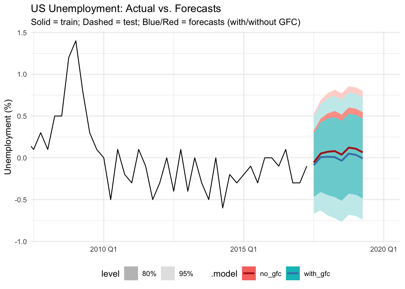
🔍 Visual Comparison & Forecast Accuracy
- Overlay actual, test (dashed), and forecast (colored) lines
- Zoom into key periods (e.g., 2008 Q1–2021 Q4) using
coord_cartesian()
- Place legend at the bottom for unobstructed viewing
- Report concise accuracy table alongside the plot
2. EDA/maps for spatio-temporal data (measles)
library(epimdr)  # For epidemic modeling functions and data
library(sf)      # For simple features support
library(tigris)  # For  US Census shapefiles as sf objects
data(dalziel)    # Load the U.S. cities measles dataset

dalziel_ts <- dalziel %>%
  as_tibble() %>%
  filter(country == "US", loc == "BALTIMORE") %>%
  mutate(
    # start-of-year date
    start_of_year = make_date(year, 1, 1),
    # each biweek is 2*(biweek-1) weeks after Jan 1
    date = start_of_year + weeks((biweek - 1) * 2)
  ) %>%
select(-start_of_year)options(tigris_use_cache = TRUE)
# get the city boundary
balt_sf <- places(state="MD", cb=TRUE) %>%
filter(NAME=="Baltimore") %>%
st_as_sf()
cases_by_year <- dalziel %>%
filter(country=="US", loc=="BALTIMORE", year %in% 1920:1948) %>%
group_by(year) %>%
summarise(
total_cases = sum(cases, na.rm=TRUE),
lon = first(lon),
lat = first(lat)
)# cross‐join to years and join cases
cases_sf <- balt_sf %>%
slice(rep(1,length(1920:1948))) %>% # duplicate geometry 4×
bind_cols(cases_by_year) # attach year & total_cases
# plot with geom_sf()
ggplot(cases_sf) +
geom_sf(aes(fill=total_cases), color="black") +
scale_fill_viridis_c(name="Cases") +
facet_wrap(~year, ncol=10, nrow = 3) +
theme_void() +
theme(strip.text = element_text(face="bold")) +
theme(legend.position = "bottom")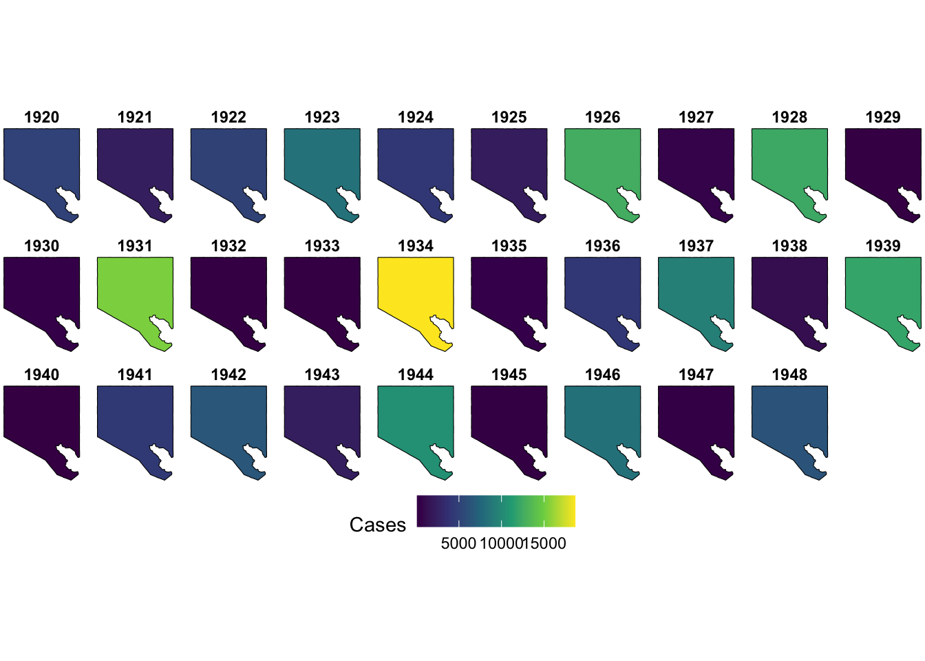
🛡️ Mitigating Data Integrity & Bias
- Ensure complete time-series coverage before forecasting 🔄
- Use consistent aggregation windows to avoid temporal bias ⏳
- Visualize both spatial and temporal dimensions together 📅🗺️
- Document data sources, cleaning steps, and assumptions 📝