Activity38

Inflation Dynamics

getSymbols("CPIAUCSL", src = "FRED", auto.assign = TRUE)

[1] "CPIAUCSL"

cpi_data <- tibble(date = index(CPIAUCSL), CPI = as.numeric(CPIAUCSL[,1])) %>%
  arrange(date) %>%
  mutate(inflation = 100 * (CPI / lag(CPI) - 1)) %>%
  mutate(Quarter = yearquarter(date)) %>% 
  as_tsibble(index = date) %>% 
  index_by(Quarter) %>% 
    summarize(CPI = mean(CPI),
              inflation = mean(inflation))

# Get US unemployment (monthly)
getSymbols("UNRATE", src = "FRED", auto.assign = TRUE)

[1] "UNRATE"

us_unemp <- data.frame(date = index(UNRATE), 
                      Unemployment = as.numeric(UNRATE$UNRATE)) %>%
  as_tsibble(index = date) %>% 
  mutate(Quarter = yearquarter(date)) %>% 
  index_by(Quarter) %>% 
    summarize(Unemployment = mean(Unemployment))


# Get US GDP (quarterly) and merge
getSymbols("GDP", src = "FRED", auto.assign = TRUE)

[1] "GDP"

us_gdp <- data.frame(date = index(GDP), GDP = as.numeric(GDP$GDP)) %>%
  as_tsibble(index = date) %>% 
  mutate(Quarter = yearquarter(date))

combined_data <- us_gdp %>% 
  inner_join(us_unemp, by = "Quarter") %>% 
  inner_join(cpi_data, by = "Quarter") %>% 
  mutate(GDP_growth = 100 * (GDP / lag(GDP) - 1)) %>% 
  dplyr::select(Quarter, date, GDP, GDP_growth, Unemployment, CPI, inflation) %>% 
  drop_na()

# View the combined data
head(combined_data) %>% knitr::kable()

Quarter	date	GDP	GDP_growth	Unemployment	CPI	inflation
1948 Q2	1948-04-01	272.567	2.5682805	3.666667	23.99333	0.9141472
1948 Q3	1948-07-01	279.196	2.4320626	3.766667	24.39667	0.2905382
1948 Q4	1948-10-01	280.366	0.4190604	3.833333	24.17333	-0.4258609
1949 Q1	1949-01-01	275.034	-1.9017998	4.666667	23.94333	-0.1942711
1949 Q2	1949-04-01	271.351	-1.3391072	5.866667	23.91667	0.0139470
1949 Q3	1949-07-01	272.889	0.5667936	6.700000	23.71667	-0.2362540

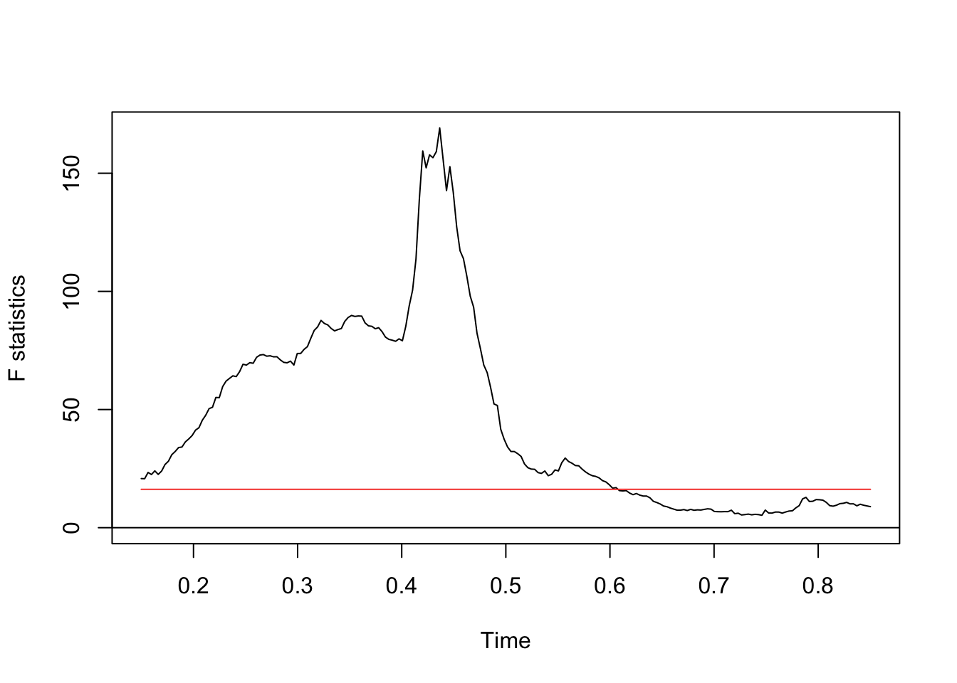
# Chow test for structural breaks
break_test <- Fstats(inflation ~ GDP_growth + Unemployment + CPI, data = combined_data)
plot(break_test)  # Identify potential breakpoints

# Estimate breakpoint date(s)
bp <- breakpoints(inflation ~  GDP_growth + Unemployment + CPI, data = combined_data)

combined_data$Quarter[bp$breakpoints] 

<yearquarter[1]>
[1] "1981 Q3"
# Year starts on: January

# Fit segmented regression
segmented_model <- lm(inflation ~ GDP_growth + Unemployment + CPI, 
                      data = combined_data, 
                      subset = breakpoints(bp)$breakpoints)

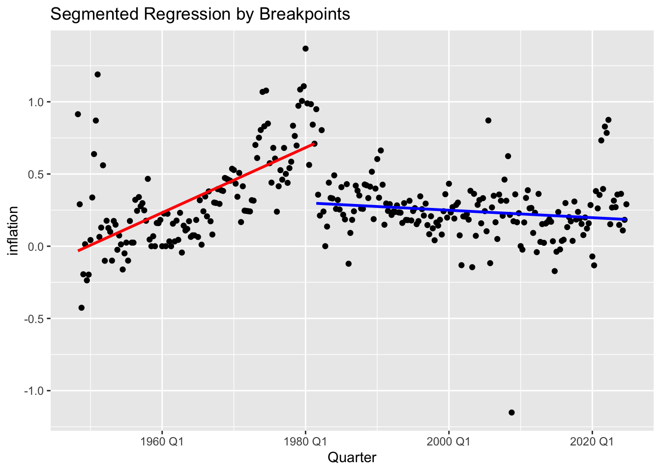
# Get breakpoint indices 
bp_indices <- bp$breakpoints 

# Split data into segments
segments <- split(combined_data, 
                 findInterval(1:nrow(combined_data), 
                              vec = c(0, bp_indices)))

# Fit models to each segment
segment_models <- lapply(segments, function(df) {
  lm(inflation ~ GDP_growth + Unemployment + CPI, data = df)
})

# Plot segmented regressions
ggplot(combined_data, aes(y =inflation, x=Quarter)) +
  geom_point() +
  geom_smooth(data = segments[[1]], method = "lm", se = FALSE, color = "red") +
  geom_smooth(data = segments[[2]], method = "lm", se = FALSE, color = "blue") +
  labs(title = "Segmented Regression by Breakpoints")

1. Fit ETS to Segments

ets_models <- segments %>% 
  map(~ {
      .x %>% 
        as_tsibble(index = Quarter) %>% 
        model(ETS(inflation))
    }
  )

ets_models %>% .[[1]] %>% report()

Series: inflation 
Model: ETS(A,N,N) 
  Smoothing parameters:
    alpha = 0.6051359 

  Initial states:
      l[0]
 0.5740484

  sigma^2:  0.0475

     AIC     AICc      BIC 
249.2322 249.4183 257.9033 

ets_models %>% .[[2]] %>% report()

Series: inflation 
Model: ETS(A,N,N) 
  Smoothing parameters:
    alpha = 0.1015893 

  Initial states:
      l[0]
 0.3795544

  sigma^2:  0.0443

     AIC     AICc      BIC 
359.3042 359.4453 368.7813 

1. Fit ARIMA to Segments

arima_models <- segments %>% 
  map(~ {
      .x %>% 
        as_tsibble(index = Quarter) %>% 
        model(ARIMA(inflation))
    }
  )

arima_models %>% .[[1]] %>% report()

Series: inflation 
Model: ARIMA(2,1,0)(0,0,2)[4] 

Coefficients:
          ar1      ar2     sma1     sma2
      -0.4293  -0.2336  -0.2345  -0.4806
s.e.   0.0908   0.0938   0.0895   0.0929

sigma^2 estimated as 0.0369:  log likelihood=30.87
AIC=-51.73   AICc=-51.26   BIC=-37.32

arima_models %>% .[[2]] %>% report()

Series: inflation 
Model: ARIMA(1,0,1)(1,0,0)[4] w/ mean 

Coefficients:
         ar1      ma1     sar1  constant
      0.8653  -0.7065  -0.0715    0.0356
s.e.  0.0957   0.1310   0.0830    0.0045

sigma^2 estimated as 0.04345:  log likelihood=27.9
AIC=-45.79   AICc=-45.44   BIC=-30

2. Fit VAR to Segments (vars)

var_models <- segments %>%
  map(~ {
      var_data <- .x %>%  as_tibble() %>% 
        dplyr::select(inflation, GDP_growth, Unemployment) %>% 
        as.data.frame()
      
      lag_order <- VARselect(var_data, type = "const")$selection["AIC(n)"]
      
      # Fit VAR model
      VAR(var_data, p = lag_order)
  })

var_models %>% .[[1]]

VAR Estimation Results:
======================= 

Estimated coefficients for equation inflation: 
============================================== 
Call:
inflation = inflation.l1 + GDP_growth.l1 + Unemployment.l1 + inflation.l2 + GDP_growth.l2 + Unemployment.l2 + inflation.l3 + GDP_growth.l3 + Unemployment.l3 + const 

   inflation.l1   GDP_growth.l1 Unemployment.l1    inflation.l2   GDP_growth.l2 
    0.485356425     0.013048892    -0.091894301     0.181597228    -0.027973849 
Unemployment.l2    inflation.l3   GDP_growth.l3 Unemployment.l3           const 
    0.027017410     0.248180381    -0.002642696     0.076192123     0.016954999 


Estimated coefficients for equation GDP_growth: 
=============================================== 
Call:
GDP_growth = inflation.l1 + GDP_growth.l1 + Unemployment.l1 + inflation.l2 + GDP_growth.l2 + Unemployment.l2 + inflation.l3 + GDP_growth.l3 + Unemployment.l3 + const 

   inflation.l1   GDP_growth.l1 Unemployment.l1    inflation.l2   GDP_growth.l2 
      1.4631099       0.1369256      -0.6840633      -0.4099621       0.1714791 
Unemployment.l2    inflation.l3   GDP_growth.l3 Unemployment.l3           const 
      1.3733278      -0.2312273      -0.1665613      -0.4515867       0.1062290 


Estimated coefficients for equation Unemployment: 
================================================= 
Call:
Unemployment = inflation.l1 + GDP_growth.l1 + Unemployment.l1 + inflation.l2 + GDP_growth.l2 + Unemployment.l2 + inflation.l3 + GDP_growth.l3 + Unemployment.l3 + const 

   inflation.l1   GDP_growth.l1 Unemployment.l1    inflation.l2   GDP_growth.l2 
     0.09656011     -0.08540808      1.41859906      0.16250345     -0.09960353 
Unemployment.l2    inflation.l3   GDP_growth.l3 Unemployment.l3           const 
    -0.81363353      0.36337053     -0.00838331      0.32764696      0.53593571 

var_models %>% .[[2]]

VAR Estimation Results:
======================= 

Estimated coefficients for equation inflation: 
============================================== 
Call:
inflation = inflation.l1 + GDP_growth.l1 + Unemployment.l1 + inflation.l2 + GDP_growth.l2 + Unemployment.l2 + const 

   inflation.l1   GDP_growth.l1 Unemployment.l1    inflation.l2   GDP_growth.l2 
    0.085879261     0.055166163     0.063392818     0.006914984     0.030556416 
Unemployment.l2           const 
   -0.060082569     0.084377774 


Estimated coefficients for equation GDP_growth: 
=============================================== 
Call:
GDP_growth = inflation.l1 + GDP_growth.l1 + Unemployment.l1 + inflation.l2 + GDP_growth.l2 + Unemployment.l2 + const 

   inflation.l1   GDP_growth.l1 Unemployment.l1    inflation.l2   GDP_growth.l2 
     0.01538228      0.82934430      1.41802522     -0.56668840      0.28639146 
Unemployment.l2           const 
    -1.29275957     -0.74656121 


Estimated coefficients for equation Unemployment: 
================================================= 
Call:
Unemployment = inflation.l1 + GDP_growth.l1 + Unemployment.l1 + inflation.l2 + GDP_growth.l2 + Unemployment.l2 + const 

   inflation.l1   GDP_growth.l1 Unemployment.l1    inflation.l2   GDP_growth.l2 
     0.10447307     -0.54363136      0.20051151      0.61151520     -0.09102577 
Unemployment.l2           const 
     0.71546509      1.11828373 

3. Model Analysis

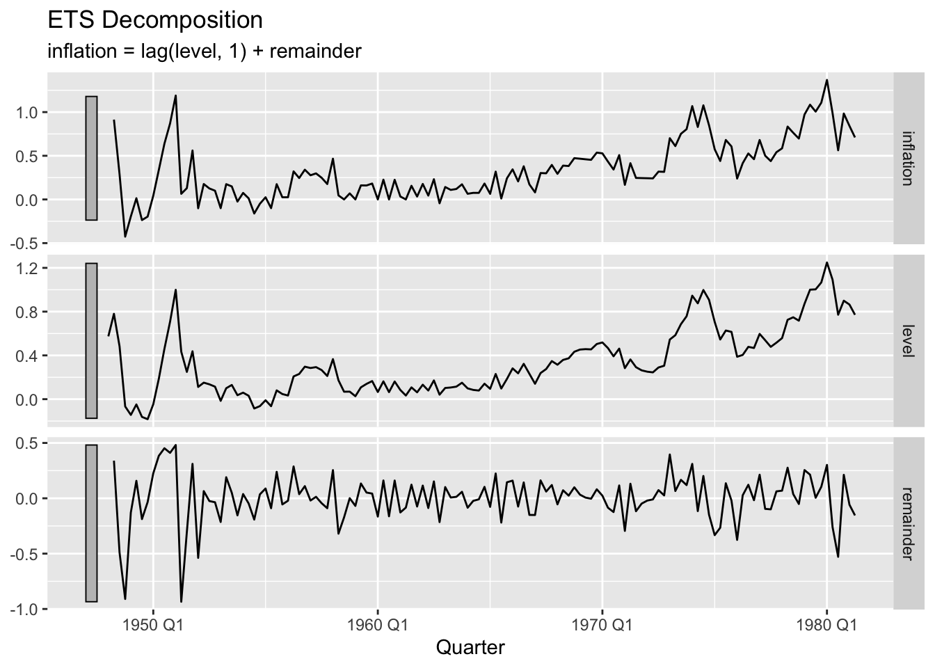
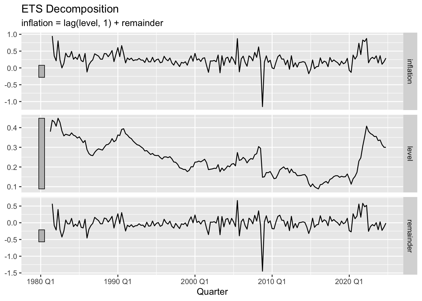
# Compare ETS components across regimes
ets_models %>% 
  compact() %>%  # Remove NULL entries
  map(~ components(.x) %>% autoplot() + labs(title = "ETS Decomposition"))

$`1`

$`2`

arima_models %>%
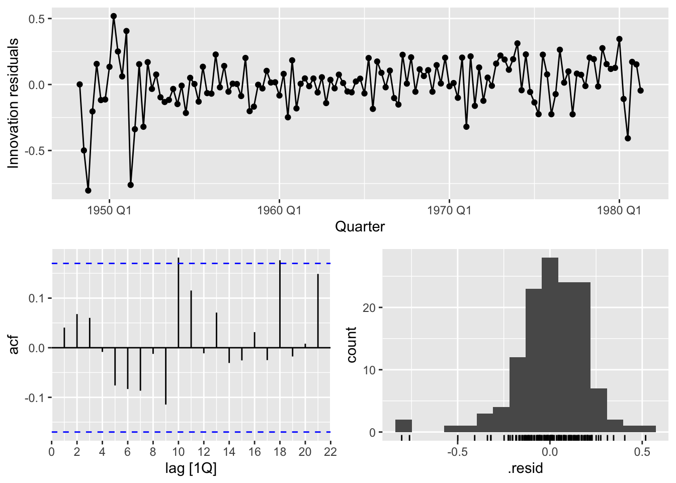
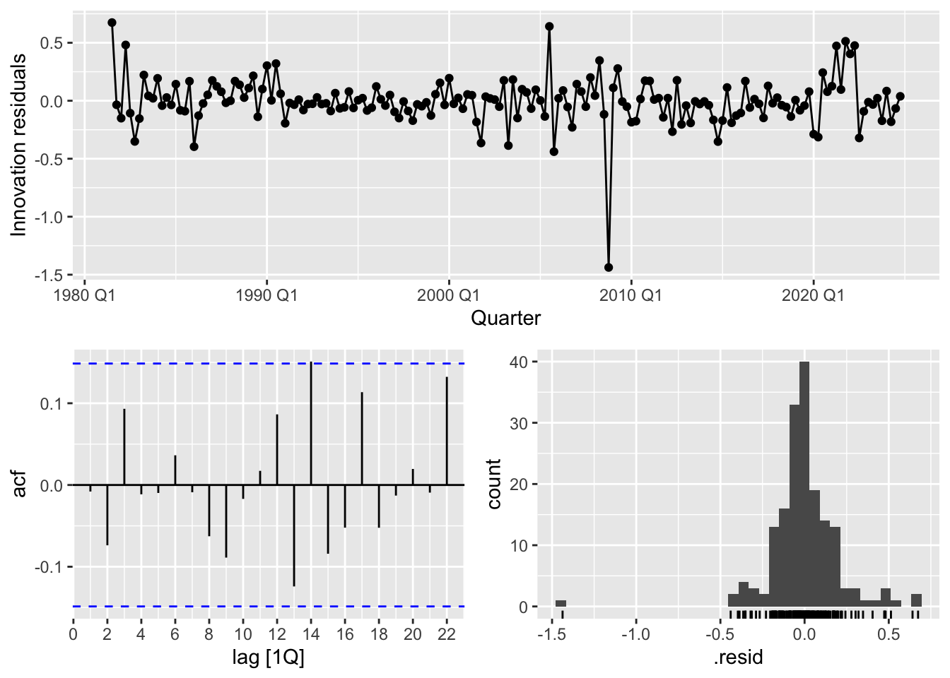
  compact() %>% .[[1]] %>% gg_tsresiduals()

arima_models %>%
  compact() %>% .[[2]] %>% gg_tsresiduals()

# Compare VAR relationships
var_models %>% 
  compact() %>% 
  map(~ {
    tibble(
      Causality_GDP = causality(.x, cause = "GDP_growth")$Granger$p.value,
      Causality_Unemp = causality(.x, cause = "Unemployment")$Granger$p.value
    )
  }) %>% knitr::kable()

Causality_GDP Causality_Unemp 0.01690187 0.004835624

Causality_GDP Causality_Unemp 5.203468e-06 6.306067e-14

Q: (Group Activity) What do these models tell us about different economic regimes before/after the breakpoints?

1. ETS

A: The analysis reveals three key regime shifts:

1. Volatility Changes (ETS):

• Pre-break: Higher \(\alpha=0.605\) (rapid adjustment to new data)
  
• Post-break: Lower \(\alpha=0.102\) (smoother evolution)

Implication: Inflation became more stable post-breakpoint
b. ARIMA

2. Structural Shifts (ARIMA):

• Pre-break: Requires differencing (\(d=1\)) with seasonal MA components
  
• Post-break: Stationary (\(d=0\)) with seasonal AR component

Implication: Fundamental change in inflation dynamics requiring different stabilization approaches

3. VAR

3. Causal Relationships (VAR):

• Pre-break: Moderate Granger-causality (GDP→inflation p=0.017; Unemp→inflation p=0.005)
  
• Post-break: Stronger causal links (GDP→inflation p=5.2e-6; Unemp→inflation p=6.3e-14)
  Implication: Post-break economic indicators became more interconnected/predictive of inflation