Activity49

Intro & Why Organization Matters

Today we’ll learn professional report structuring in R Markdown. Key goals:

• Clean main text with >hidden code

• >Appendix for reproducibility
  

• >Optimized figures/tables with captions
  

• Logical >markdown headings”

Basic Chunk Management

```{r setup, include=FALSE}
# Libraries, data load, functions here
knitr::opts_chunk$set(echo=FALSE, message=FALSE)
```

Add a figure caption

```{r fig_main, fig.cap="Main time series plot"}
p_main  # Plot object from your code
```

Key points:

• >include=FALSE hides setup code completely
  
• >echo=FALSE shows output without code
  
• Always use >fig.cap for figures

Advanced Figure/Table Formatting

```{r model_table, results='asis'}
knitr::kable(model_comparison, caption="Model accuracy comparison")
```

```{r decomposition, fig.cap="STL decomposition", fig.width=8, fig.height=5}
p_stl  # Your decomposition plot
```

Table/figures:

• >kable(caption = “A nice caption”) for tables with captions
  
• >fig.width/height adjustments
  
• >results=‘asis’ for proper table rendering

Residual Diagnostics Section

Diagnostics

```{r residuals, fig.cap="ARIMA residuals", fig.subcap=c("TS", "ACF", "Hist")}
arima_fit %>% gg_tsresiduals()  
```

Emphasize:

• >Multi-panel figures with subcaptions
  
• Consistent >theme_minimal usage
  
• Interpretation in text near figures

Appendix Creation

```{r appendix_code, echo=TRUE}
# Smaller chunks, with informative comments
trends_ufo %>% autoplot()  # Original plotting code
```

Critical skills

• >eval=FALSE prevents duplicate computation
  
• Organized >code documentation

Final Polish

• Show >heading hierarchy: # Section > ## Subsection
  
• Demonstrate >global chunk options in setup

Cheatsheet:

Essential Chunk Options:
• echo=FALSE       - Hide code
• include=FALSE    - Run but hide everything
• fig.cap="Text"   - Figure captions
• results='asis'   - For tables
• fig.width=8      - Control plot size
• eval=FALSE       - Show code without running

Class Activity

Create a well-organized skeletal report analyzing UFO search Trends in US using R Markdown. Your report must:
- Separate code execution from presentation using include=FALSE for setup/data chunks and echo=FALSE for result displays
- Show all figures/tables in the main text with descriptive captions (fig.cap/kable(caption=))
- Include full reproducible code in an Appendix using eval=FALSE, echo=TRUE
- Compare models professionally with knitr::kable() formatted tables
- Structure content clearly under these headings: Introduction, Results (Trends/Models), Diagnostics, Appendix

Practice report-writing skills by:

1. Keeping the main text code-free while showing visualizations
   
2. Using chunk labels consistently (e.g., fig_main, tbl_models)
   
3. Cross-referencing appendix code to main text elements
   
4. Optimizing figure sizes via fig.width/height

multiTimelineUFO <- read_csv("data/multiTimelineUFO.csv", skip = 1)
trends_ufo <- multiTimelineUFO %>% 
  janitor::clean_names() %>% 
  mutate(month = yearmonth(month)) %>% 
  rename(hits = ufo_united_states) %>% 
  as_tsibble(index = month)

Introduction

Methodology

Results

Main Trends

trends_ufo %>% autoplot(hits) +
  labs(y = "Relative Interest (0-100)", x = "Month") +
  theme_minimal()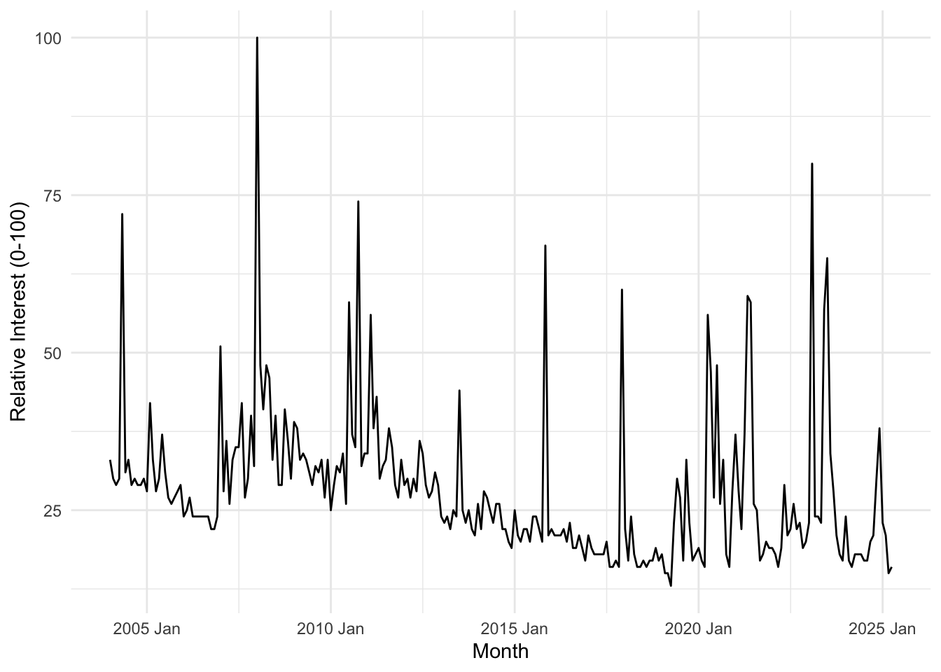

Google Trends Interest in UFOs (2004-2023)

Model Comparisons

arima_fit <- trends_ufo %>% model(ARIMA(hits))
lambda_est <- trends_ufo %>% features(hits, guerrero) %>% pull(lambda_guerrero)
arima_fit_bc <- trends_ufo %>% model(ARIMA(box_cox(hits, lambda_est)))
ets_fit_bc <- trends_ufo %>% model(ETS(box_cox(hits, lambda_est)))

model_comparison <- accuracy(arima_fit_bc) %>%
  bind_rows(accuracy(ets_fit_bc)) %>% 
  bind_rows(accuracy(arima_fit))
knitr::kable(model_comparison, caption = "Model Accuracy Metrics Comparison")

Model Accuracy Metrics Comparison

.model	.type	ME	RMSE	MAE	MPE	MAPE	MASE	RMSSE	ACF1
ARIMA(box_cox(hits, lambda_est))	Training	0.6205578	10.58485	5.845902	-5.234272	18.13860	0.6410787	0.6970692	-0.0440546
ETS(box_cox(hits, lambda_est))	Training	0.6623999	10.65716	5.843008	-4.918688	18.20439	0.6407613	0.7018310	0.0625724
ARIMA(hits)	Training	-0.4361228	10.64533	6.422410	-9.764741	21.20102	0.7043002	0.7010519	-0.0077131

Diagnostics

ARIMA and ETS Residuals

arima_fit %>% gg_tsresiduals()
ets_fit_bc %>% gg_tsresiduals()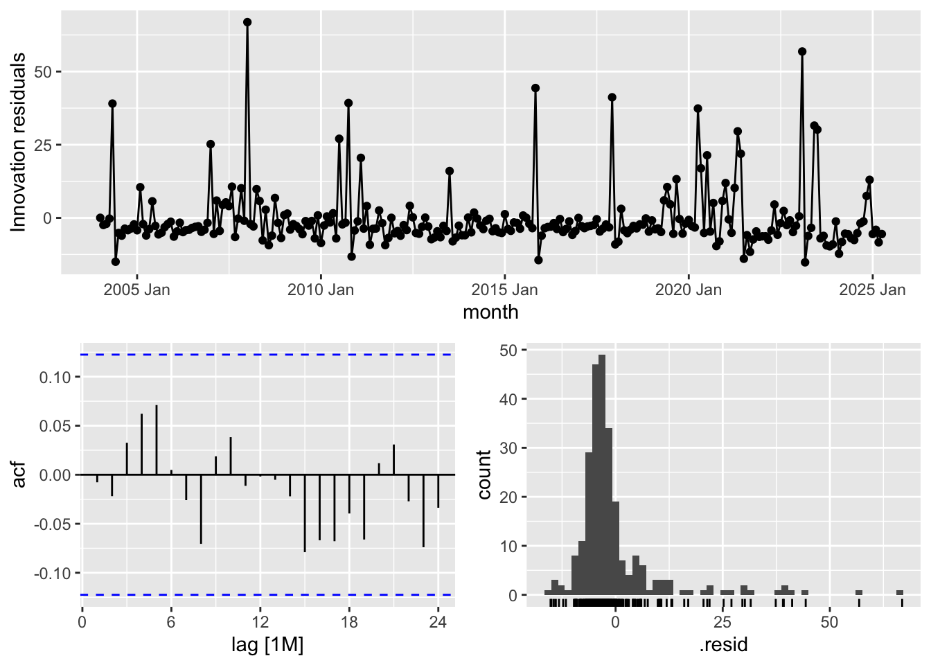

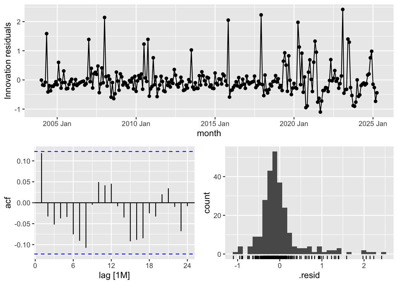
ARIMA

ETS

Residual Diagnostics for ARIMA and ETS Models

Appendix

R-Code Listing