Activity40

Modeling U.S. Inflation Dynamics: A Time Series Application

This analysis investigates U.S. inflation dynamics using quarterly CPI, unemployment, and GDP data from FRED. Inflation is defined as the quarterly percentage change in CPI:
\[\text{inflation}_t = 100 \times \left(\frac{CPI_t}{CPI_{t-1}} - 1\right)\]

The modeling strategy integrates traditional time series approaches (AR and ARIMA) with structural diagnostics and modern multivariate frameworks to evaluate the influence of macroeconomic variables on inflation. Let’s get the data first:

getSymbols("CPIAUCSL", src = "FRED", auto.assign = TRUE)

[1] "CPIAUCSL"

cpi_data <- tibble(date = index(CPIAUCSL), CPI = as.numeric(CPIAUCSL[,1])) %>%
  arrange(date) %>%
  mutate(inflation = 100 * (CPI / lag(CPI) - 1)) %>%
  mutate(Quarter = yearquarter(date)) %>% 
  as_tsibble(index = date) %>% 
  index_by(Quarter) %>%
  summarize(CPI = mean(CPI), inflation = mean(inflation))

getSymbols("UNRATE", src = "FRED", auto.assign = TRUE)

[1] "UNRATE"

us_unemp <- data.frame(date = index(UNRATE), Unemployment = as.numeric(UNRATE$UNRATE)) %>%
  as_tsibble(index = date) %>%
  mutate(Quarter = yearquarter(date)) %>%
  index_by(Quarter) %>%
  summarize(Unemployment = mean(Unemployment))

getSymbols("GDP", src = "FRED", auto.assign = TRUE)

[1] "GDP"

us_gdp <- data.frame(date = index(GDP), GDP = as.numeric(GDP$GDP)) %>%
  as_tsibble(index = date) %>%
  mutate(Quarter = yearquarter(date))

economic_data <- us_gdp %>%
  inner_join(us_unemp, by = "Quarter") %>%
  inner_join(cpi_data, by = "Quarter") %>%
  mutate(GDP_growth = 100 * (GDP / lag(GDP) - 1)) %>%
  dplyr::select(Quarter, date, GDP, GDP_growth, Unemployment, CPI, inflation) %>%
  tidyr::drop_na()

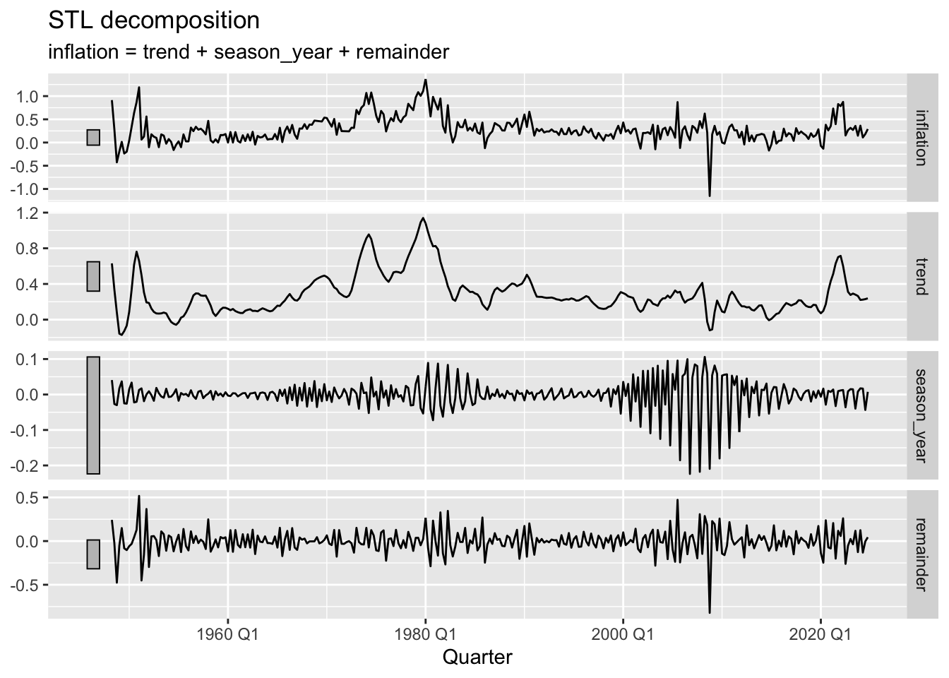
STL decomposition of the inflation series reveals clear seasonal and cyclical behavior. This reinforces the use of seasonal components in ARIMA models and motivates further refinement using explicitly seasonal structures.

economic_data %>%
  as_tsibble(index = Quarter) %>%
  model(STL(inflation ~ trend() + season())) %>%
  components() %>%
  autoplot()

Step 1: AR(1) Regression

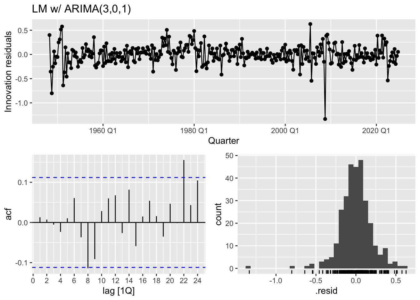
We begin with an autoregressive model including lagged inflation, unemployment, and GDP growth. Residual diagnostics reveal no significant autocorrelation, implying the AR(1) structure is sufficient to capture temporal dependencies.

The model is of the form:

\[ \text{Inflation}_t = \beta_0 + \beta_1 \cdot \text{GDP\_growth}_t + \beta_2 \cdot \text{Unemployment}_t + \eta_t \]

where \(( \eta_t \sim \text{ARIMA}(3,0,1)).\)

arima_model <- economic_data %>%
  as_tsibble(index = Quarter) %>%
  model(ARIMA(inflation ~ GDP_growth + Unemployment))

report(arima_model)

Series: inflation 
Model: LM w/ ARIMA(3,0,1) errors 

Coefficients:
         ar1     ar2     ar3      ma1  GDP_growth  Unemployment  intercept
      0.6260  0.0543  0.1793  -0.3189      0.0398       -0.0335     0.4109
s.e.  0.2307  0.1048  0.0996   0.2395      0.0099        0.0150     0.1033

sigma^2 estimated as 0.04254:  log likelihood=52.18
AIC=-88.36   AICc=-87.88   BIC=-58.55

arima_model %>% 
  residuals() %>% 
  features(.resid, ~ljung_box(.x, lag = 10)) %>% 
  knitr::kable()

.model	lb_stat	lb_pvalue
ARIMA(inflation ~ GDP_growth + Unemployment)	8.922994	0.5394271

The Ljung-Box diagnostics show no strong autocorrelation, indicating the AR(1) structure with regressors reasonably captures short-term dynamics.

Step 2: ARIMA-X Model

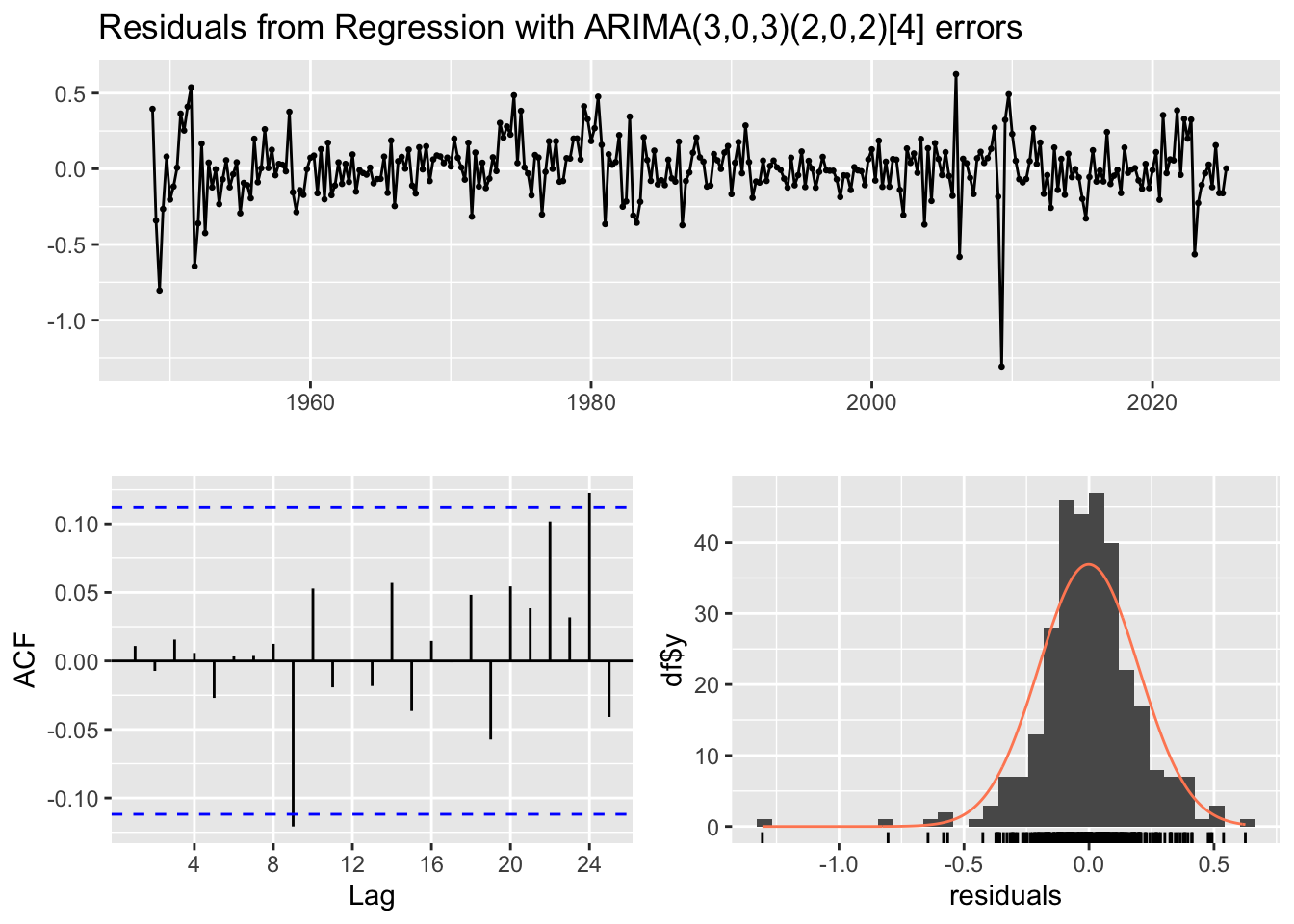
We improve upon this by fitting an ARIMA model with exogenous regressors using forecast::auto.arima(), which also allows for seasonal ARMA components. The best-fit specification is an ARIMA(3,0,3)(2,0,2)[4], indicating both short- and medium-term seasonal effects.

This yields a model of the form:

\[ \text{Inflation}_t = \beta_0 + \beta_1 \cdot \text{GDP\_growth}_t + \beta_2 \cdot \text{Unemployment}_t + \eta_t \]

where \((\eta_t \sim \text{ARIMA}(3,0,3)(2,0,2)_4)\).

library(forecast)
xreg_matrix <- economic_data %>% as_tibble() %>% 
  dplyr::select(GDP_growth, Unemployment) %>%
  data.matrix()

start_year <- year(min(economic_data$Quarter))
start_month <- month(min(economic_data$Quarter))
inflation_ts <- ts(economic_data$inflation, frequency = 4, start = c(start_year, start_month))

arimax_model <- auto.arima(inflation_ts, xreg = xreg_matrix)

summary(arimax_model)

Series: inflation_ts 
Regression with ARIMA(3,0,3)(2,0,2)[4] errors 

Coefficients:
          ar1     ar2     ar3     ma1     ma2      ma3     sar1     sar2
      -0.3160  0.2542  0.8826  0.6122  0.1032  -0.5369  -0.3004  -0.0796
s.e.   0.0779  0.0569  0.0726  0.1158  0.0978   0.1127   0.3286   0.2993
        sma1     sma2  intercept  GDP_growth  Unemployment
      0.3459  -0.1138     0.4139      0.0355       -0.0328
s.e.  0.3350   0.3070     0.1031      0.0097        0.0139

sigma^2 = 0.04171:  log likelihood = 58
AIC=-88   AICc=-86.56   BIC=-35.82

Training set error measures:
                       ME      RMSE       MAE       MPE     MAPE      MASE
Training set -0.001319576 0.1998711 0.1407113 -5006.591 5083.211 0.6846118
                  ACF1
Training set 0.0108953

arimax_model %>% 
  residuals() %>% 
  ljung_box(lag = 10) %>% 
  knitr::kable()

	x
lb_stat	5.9605728
lb_pvalue	0.8185648

The Ljung-Box gives us larger p-value this time, and the residuals should be more like white noise.

Activity 1: Write model equations for the ARIMA model in Step 1

The fitted model is a linear regression with ARIMA(3,0,1) errors, often called an ARIMA with exogenous regressors (ARIMAX). The equation form is:

\[\begin{aligned} \text{inflation}_t &= \beta_0 + \beta_1 \cdot \text{GDP\_growth}_t + \beta_2 \cdot \text{Unemployment}_t + \eta_t \\ \eta_t &= \phi_1 \eta_{t-1} + \phi_2 \eta_{t-2} + \phi_3 \eta_{t-3} + \theta_1 \varepsilon_{t-1} + \varepsilon_t \\ \varepsilon_t &\sim \text{WN}(0, \sigma^2) \end{aligned}\]

Where:

• \(\beta_1 = 0.0398\) (GDP growth has a positive effect)
• \(\beta_2 = -0.0335\) (unemployment has a negative effect)
• \(\phi_1, \phi_2, \phi_3\) are AR terms
• \(\theta_1\) is the MA(1) term
• \(\sigma^2 = 0.04254\) is the estimated variance of white noise

The intercept (\(0.411\)) represents baseline inflation when GDP growth and unemployment are zero—an extrapolation. The AR(3) coefficients collectively dampen long-term deviations from this baseline, while the MA(1) term absorbs shocks.

Activity 2: Residual Diagnostics

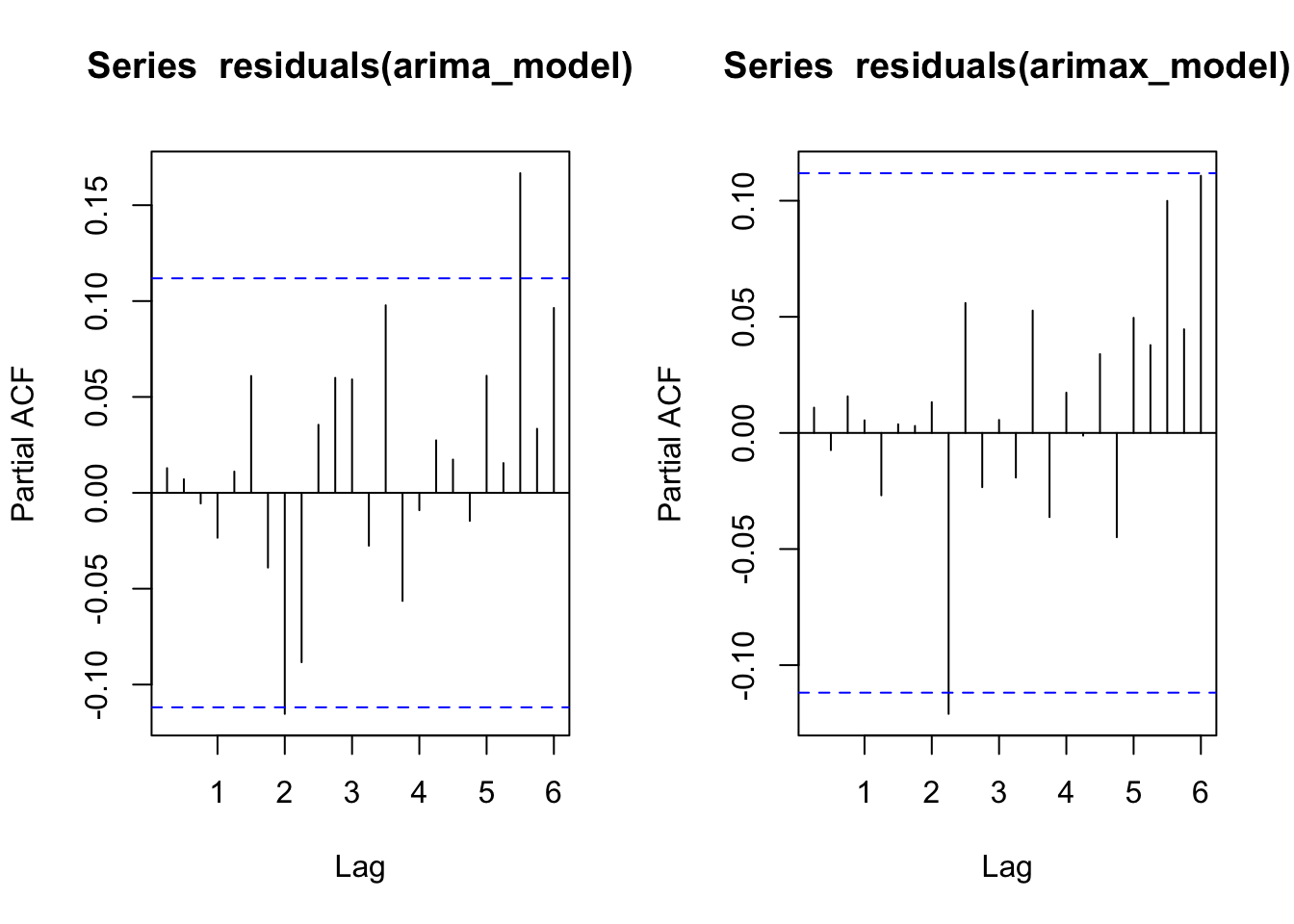
Examine ACF/PACF plots and Ljung-Box test results for the ARIMA model. Interpret residual autocorrelation and explain why traditional AR(1) structures may fail in macroeconomic contexts.

library(gridExtra)
gg_tsresiduals(arima_model) + ggtitle("LM w/ ARIMA(3,0,1)")

checkresiduals(arimax_model) 

    Ljung-Box test

data:  Residuals from Regression with ARIMA(3,0,3)(2,0,2)[4] errors
Q* = 6.1871, df = 3, p-value = 0.1029

Model df: 10.   Total lags used: 13

par(mfrow = c(1,2))
pacf(residuals(arima_model), lag.max = 24) 
pacf(residuals(arimax_model), lag.max = 24) 

Both models exhibit residual independence (p > 0.05), but the higher p-value for the seasonal ARIMA model (0.819) indicates superior white noise.

Activity 3: Variable Transformation

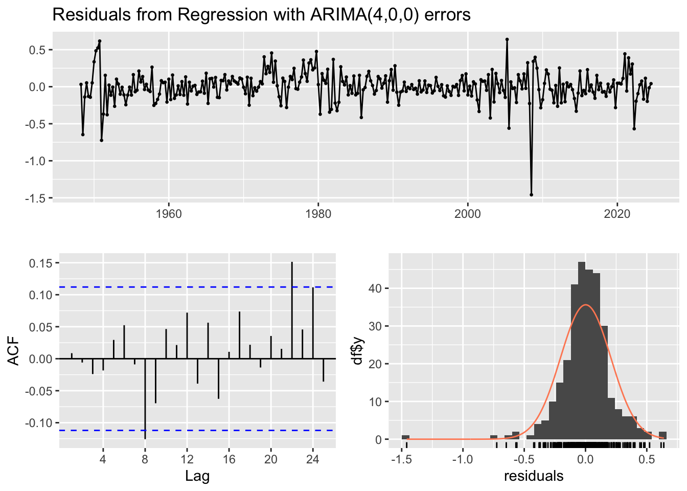
To address potential nonstationarity and heteroskedasticity, GDP is log-transformed and unemployment is differenced. An ARIMA(4,0,0) model with these transformed covariates yields a competitive AIC and improved interpretability. What do the results suggests? Why are the transformations needed?

• Log(GDP) is positively associated with inflation.
• Changes in unemployment are negatively associated with inflation.

These transformations help stabilize variance and center the series around a constant mean.

economic_data <- economic_data %>%
  mutate(log_GDP = log(GDP),
         delta_Unemployment = difference(Unemployment)) %>%
  drop_na()

arima_transformed <- Arima(
  ts(economic_data$inflation, frequency = 4, start = c(1948, 2)),
  order = c(4, 0, 0),
  xreg = cbind(log_GDP = economic_data$log_GDP,
               delta_Unemployment = economic_data$delta_Unemployment)
)

summary(arima_transformed)

Series: ts(economic_data$inflation, frequency = 4, start = c(1948, 2)) 
Regression with ARIMA(4,0,0) errors 

Coefficients:
         ar1     ar2     ar3      ar4  intercept  log_GDP  delta_Unemployment
      0.3512  0.1753  0.2749  -0.0209     0.1994   0.0092             -0.0340
s.e.  0.0579  0.0596  0.0594   0.0584     0.2932   0.0354              0.0154

sigma^2 = 0.04305:  log likelihood = 50.18
AIC=-84.36   AICc=-83.87   BIC=-54.57

Training set error measures:
                      ME      RMSE       MAE      MPE    MAPE      MASE
Training set 0.001433048 0.2050985 0.1427111 -4527.97 4608.29 0.7022001
                    ACF1
Training set 0.008634326

checkresiduals(arima_transformed)

    Ljung-Box test

data:  Residuals from Regression with ARIMA(4,0,0) errors
Q* = 6.4755, df = 4, p-value = 0.1663

Model df: 4.   Total lags used: 8

Differencing unemployment stabilizes its variance by removing a unit root, transforming a non-stationary series into a stationary one. This allows the coefficient on \(\Delta\text{Unemployment}\) (-0.034) to represent the change in labor market conditions. Similarly, log-transforming GDP linearizes its exponential growth trend, reducing changing variance.

Activity 4: VAR model

Write the model equation for inflation in terms of the following VAR model output and interpret it.

library(vars)
var_data <- economic_data %>% as_tibble() %>% 
  tidyr::drop_na() %>% 
  dplyr::select(inflation, GDP_growth, delta_Unemployment)

lag_order <- VARselect(var_data, type = "const")$selection["AIC(n)"]
var_model <- VAR(var_data, p = lag_order)
summary(var_model$varresult$inflation)

Call:
lm(formula = y ~ -1 + ., data = datamat)

Residuals:
     Min       1Q   Median       3Q      Max 
-1.38107 -0.09893 -0.00104  0.09479  0.63060 

Coefficients:
                      Estimate Std. Error t value Pr(>|t|)    
inflation.l1           0.28733    0.05904   4.867 1.85e-06 ***
GDP_growth.l1          0.02681    0.01558   1.720  0.08641 .  
delta_Unemployment.l1  0.02672    0.02548   1.049  0.29525    
inflation.l2           0.11125    0.06018   1.849  0.06553 .  
GDP_growth.l2          0.01770    0.01628   1.087  0.27804    
delta_Unemployment.l2  0.01155    0.02710   0.426  0.67026    
inflation.l3           0.19814    0.05969   3.320  0.00102 ** 
GDP_growth.l3          0.04183    0.01614   2.591  0.01004 *  
delta_Unemployment.l3  0.04544    0.02608   1.742  0.08248 .  
const                 -0.01775    0.02940  -0.604  0.54648    
---
Signif. codes:  0 '***' 0.001 '**' 0.01 '*' 0.05 '.' 0.1 ' ' 1

Residual standard error: 0.2016 on 293 degrees of freedom
Multiple R-squared:  0.474, Adjusted R-squared:  0.4578 
F-statistic: 29.34 on 9 and 293 DF,  p-value: < 2.2e-16

stringr::str_glue("AIC:", {AIC(var_model$varresult$inflation)})

AIC:-98.7910159323021

This yields a model of the form:

\[\begin{aligned} \text{inflation}_t &= \alpha_0 + \alpha_1 \cdot \text{inflation}_{t-1} + \alpha_2 \cdot \text{GDP\_growth}_{t-1} + \alpha_3 \cdot \Delta \text{Unemployment}_{t-1} \\ &\quad + \alpha_4 \cdot \text{inflation}_{t-2} + \alpha_5 \cdot \text{GDP\_growth}_{t-2} + \alpha_6 \cdot \Delta \text{Unemployment}_{t-2} \\ &\quad + \alpha_7 \cdot \text{inflation}_{t-3} + \alpha_8 \cdot \text{GDP\_growth}_{t-3} + \alpha_9 \cdot \Delta \text{Unemployment}_{t-3} + \varepsilon_t \end{aligned}\]

where \(\varepsilon_t \sim \text{WN}(0, \sigma^2)\), and lag order \(p=3\) was selected by AIC.

Inflation’s strongest predictor is its first lag (\(\hat{\alpha}_1 = 0.287\)), indicating momentum from recent price changes. The delayed GDP growth effects (significant at lags 1 and 3) suggest that economic expansions influence inflation through staggered channels—e.g., initial demand surges (lag 1) followed by capacity constraints (lag 3). Unemployment changes exhibit mixed significance, with lag 3’s positive coefficient (\(0.045\)) implying that sustained labor market improvements may eventually fuel inflationary expectations.