Activity41

Structural Breaks in COVID-19 Data

The COVID-19 pandemic created distinct epidemiological regimes where parameters governing case growth changed fundamentally. Identifying these structural breaks through vaccine rollouts, policy changes, and variant emergence helps quantify intervention effectiveness and improve forecasting. This case study demonstrates how to detect and model regime shifts using FDA emergency vaccine authorization (Jan 2021) as a natural experiment.

\[ \begin{aligned} \text{Confirmed}_t &= \underbrace{\phi_0 + \phi_1 \text{Confirmed}_{t-1}}_{\text{Autoregressive component}} + \underbrace{\beta \text{Vaccines}_t}_{\text{Current vaccines}} + \underbrace{\gamma D_t}_{\text{Break effect}} + \epsilon_t \\ D_t &= \begin{cases} 1 & \text{if } t \geq \tau \ (\text{post-break}) \\ 0 & \text{otherwise} \end{cases} \\ \epsilon_t &\sim \text{WN}(0, \sigma^2) \end{aligned} \]

Data Preparation

# Retrieve COVID-19 data for the United States and prepare a tsibble
# Get cumulative COVID metrics
covid_raw <- covid19(country = "US", level = 1, verbose = FALSE) %>%
  as_tsibble(index = date) %>%
  select(date, confirmed, people_vaccinated) %>%
  rename(vaccines = people_vaccinated)

We first convert raw cumulative COVID-19 data to new weekly cases/vaccinations using lagged differences. Log-transformation stabilizes variance while preserving relative changes. Weekly aggregation reduces daily reporting noise (e.g., weekend under-reporting).

# Convert to NEW weekly cases 
covid_weekly <- covid_raw %>%
  mutate(across(c(confirmed, vaccines), ~. - lag(.))) %>% # Calculate daily changes
  index_by(week = yearweek(date)) %>%
  summarize(
    cases = sum(confirmed, na.rm = TRUE),
    vaccines = sum(vaccines, na.rm = TRUE)
  ) %>%
  filter(cases > 0, vaccines >= 0) %>%
  mutate(across(c(cases, vaccines), ~ log(. + 1))) 

Activity 1: Visual Break Identification

covid_weekly %>% as_tibble() %>% 
  pivot_longer(-week) %>%
  ggplot(aes(week, value)) +
  geom_line() +
  geom_vline(
    xintercept = as.Date(yearweek("2021-01-11")), 
    color = "red",
    linetype = "dashed"
  ) +
  facet_grid(name ~ ., scales = "free") +
  labs(
    title = "U.S. COVID Trends with Vaccine Breakpoint Hypothesis",
    subtitle = "Red line marks FDA emergency vaccine approval date"
  )

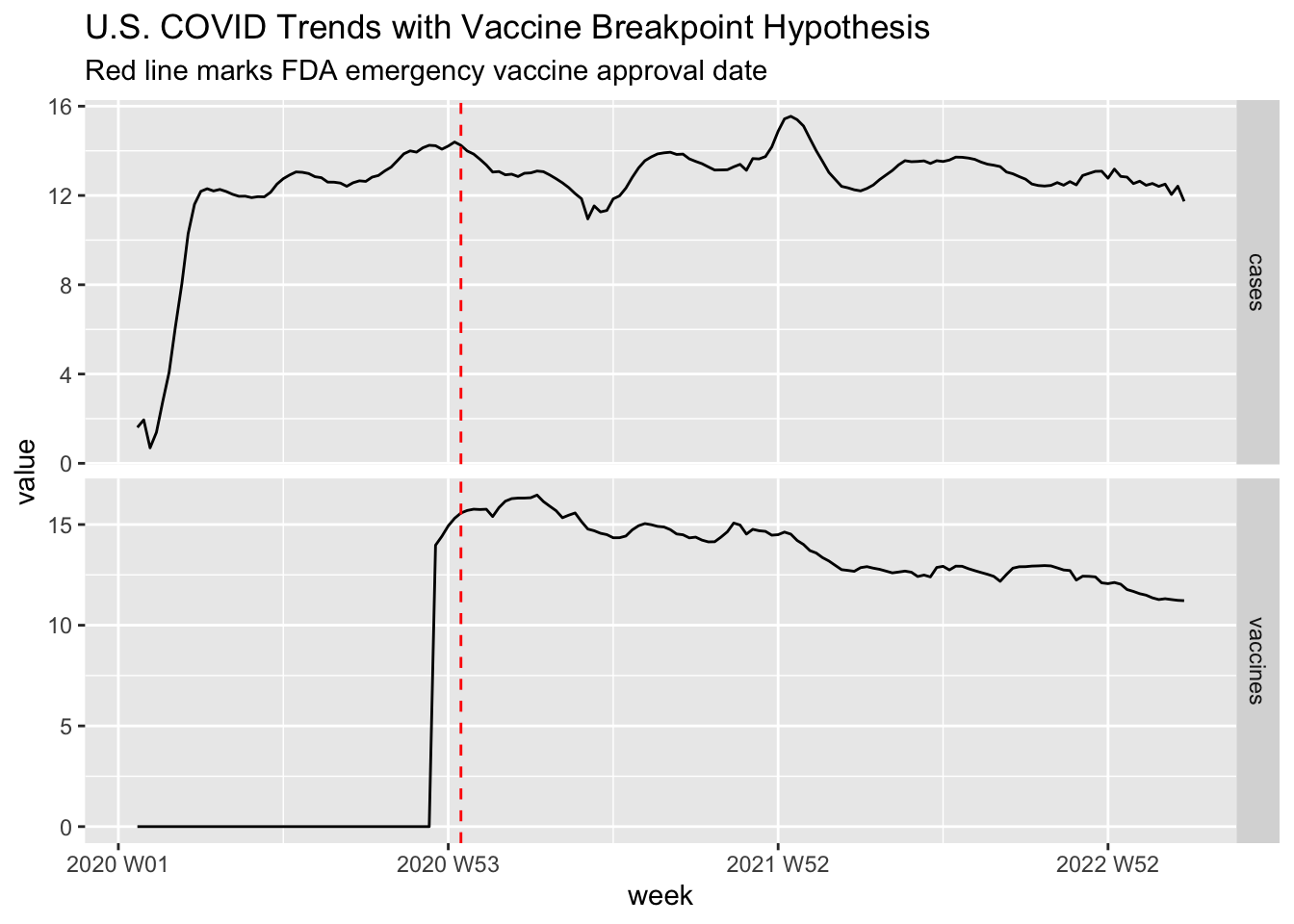
The vertical line marks January 2021 when vaccines became widely available. Visual analysis suggests a potential structural break - case growth deceleration post-vaccination despite similar transmission conditions.

Activity 2: Formal Breakpoint Test

library(strucchange)
bp_test <- Fstats(cases ~ vaccines, data = covid_weekly)

bp_cases <- breakpoints(cases ~ 1, data = covid_weekly, h = 0.15)
break_week <- covid_weekly$week[bp_cases$breakpoints]

# Create regime dummy
covid_weekly <- covid_weekly %>% 
  mutate(post_vax = (week >= break_week) %>% as.integer())

Key Equation: Structural Break Model

\[ \begin{aligned} \log \left(\text { Cases }_t\right)&=\phi_0+\phi_1 \log \left(\text { Cases }_{t-1}\right)+\beta \log \left(\text { Vaccines }_t\right)+\gamma D_t+\epsilon_t \\ \text{where } D_t &= \begin{cases} 0 & \text{pre-vaccine} \\ 1 & \text{post-vaccine} \end{cases} \end{aligned} \] ## Activity 3: Modeling and Forecasting with Breaks

library(forecast)

# Convert to ts objects
cases_ts <- ts(covid_weekly$cases, 
              frequency = 52,
              start = yearweek(min(covid_weekly$week)))

xreg_matrix <- covid_weekly %>% as_tibble() %>% 
  select(vaccines, post_vax) %>%
  mutate(post_vax = as.numeric(post_vax)) %>%
  data.matrix()

# Auto-ARIMAX
arimax_forecast <- auto.arima(
  cases_ts,
  xreg = xreg_matrix
)

arimax_forecast %>% summary()

Series: cases_ts 
Regression with ARIMA(4,0,2)(1,0,0)[52] errors 

Coefficients:
         ar1      ar2      ar3     ar4      ma1     ma2    sar1  intercept
      2.1919  -1.0385  -0.6612  0.5042  -0.9009  0.2029  0.0401    11.2746
s.e.  0.1279   0.3349   0.3368  0.1235   0.1331  0.1815  0.1069     1.9063
      vaccines  post_vax
       -0.0022    0.0500
s.e.    0.0172    0.2381

sigma^2 = 0.08649:  log likelihood = -30.56
AIC=83.12   AICc=84.83   BIC=117.35

Training set error measures:
                     ME      RMSE       MAE        MPE     MAPE      MASE
Training set 0.02989448 0.2850902 0.1778063 -0.6505711 3.342386 0.1153798
                    ACF1
Training set -0.01963548

# Residual diagnostics
arimax_forecast %>% 
  checkresiduals()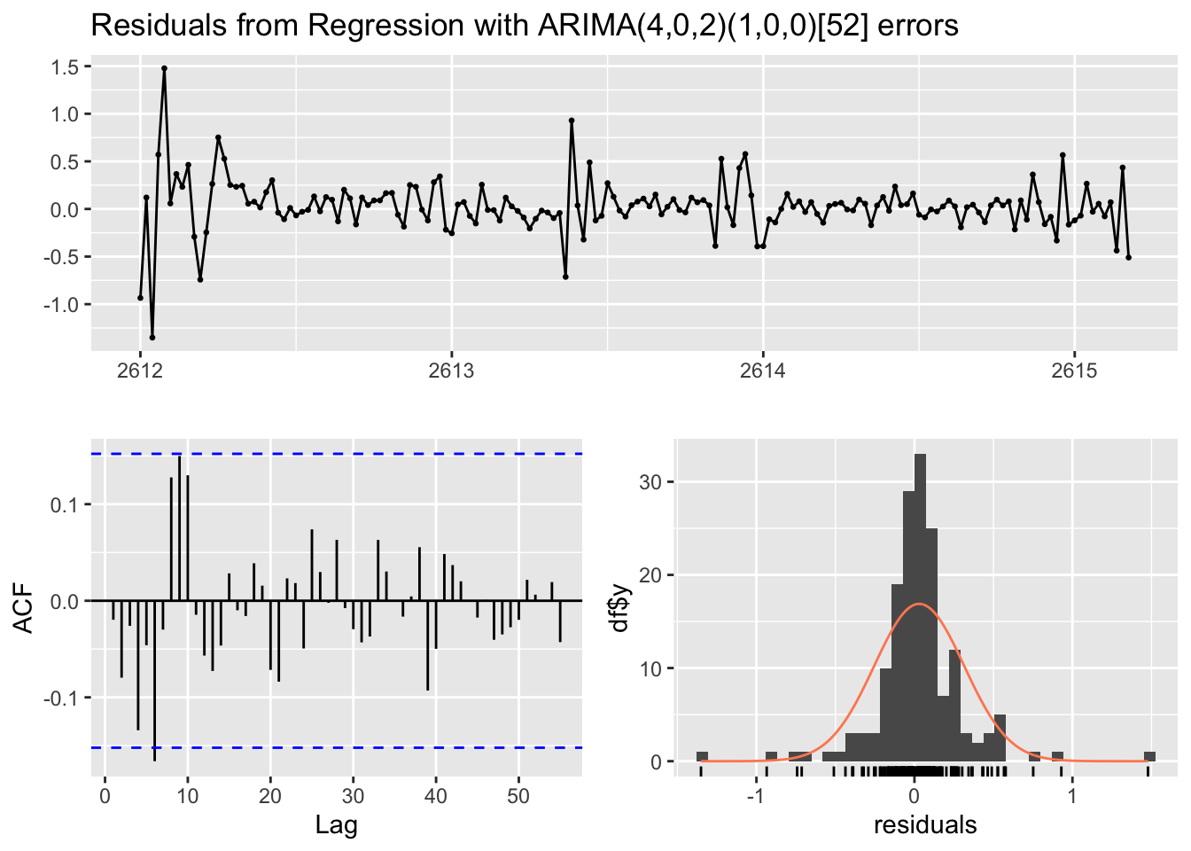

    Ljung-Box test

data:  Residuals from Regression with ARIMA(4,0,2)(1,0,0)[52] errors
Q* = 28.818, df = 26, p-value = 0.3194

Model df: 7.   Total lags used: 33

arimax_forecast %>% 
  residuals() %>% 
  ljung_box(lag = 10) %>% 
  knitr::kable()

	x
lb_stat	19.5685060
lb_pvalue	0.0336084

Questions

Q1: Why did we use both visual inspection and formal Chow tests to identify structural breaks?

Q2: Why does weekly aggregation help with structural break detection despite losing temporal granularity?

(Hint: Consider surveillance reporting cycles and weekend effects)

Q3: The original analysis uses vaccine administration as a break source. Propose 3 alternative candidate breakpoints from pandemic history and operationalize their measurement.

Q4: How would you interpret a positive coefficient (0.0182) on the post-vaccine dummy variable?

Q5 : Modify the breakpoint code to test for two or more structural breaks (pre/during/post vaccine eras).

# Solution:
bp_multi <- breakpoints(cases ~ 1 + vaccines, data = covid_weekly, h = 0.02, breaks = 5)
regimes <- covid_weekly$week[bp_multi$breakpoints]
regimes

<yearweek[5]>
[1] "2020 W08" "2020 W11" "2020 W43" "2021 W06" "2021 W29"
# Week starts on: Monday

\[ \begin{aligned} \log(\text{Cases}_t) &= \phi_0 + \sum_{k=1}^k \gamma_k D_t^{(k)} + \beta_t \log(\text{Vaccines}_t) \end{aligned} \]