Activity12

Model Selection & Diagnostic Criteria

Today, we will walk through a complete model selection exercise using VIX data. Our goals are to:

Perform Exploratory Data Analysis (EDA) with visual diagnostics.
Fit built-in models (ARIMA and ETS) using the Tidyverts framework.
Evaluate models based on five metrics: AIC, AICc, BIC, Mean Squared Error (MSE), and Root Mean Squared Error (RMSE).
Conclude on the optimal model by comparing these metrics along with residual diagnostics and forecast performance.

For a model with \(n\) observations and \(k\) parameters (including the intercept), the evaluation criteria are defined as:

\[ \begin{align} \text{AIC} &= n\ln\left(\frac{\text{RSS}}{n}\right) + 2k,\\[1mm] \text{BIC} &= n\ln\left(\frac{\text{RSS}}{n}\right) + k\ln(n),\\[1mm] \text{AICc} &= \text{AIC} + \frac{2k(k+1)}{n-k-1}, \end{align} \]

and the error metrics:

\[ \begin{align} \text{MSE} &= \frac{\text{RSS}}{n},\\[1mm] \text{RMSE} &= \sqrt{\text{MSE}}. \end{align} \]

Data Preparation

We retrieve the VIX data and format as a tsibble, handling missing values while preserving the original adjusted price series.

# Retrieve VIX data from 2000-01-01 to current date and convert to a tsibble
vix_data <- tq_get("^VIX", from = "2000-01-01", 
                   to = "2025-01-01", 
                   get = "stock.prices") %>% 
  as_tsibble(index = date)

# Clean and interpolate missing values
vix_data <- vix_data %>% 
  tsibble::fill_gaps() %>% 
  mutate(adjusted = zoo::na.approx(adjusted)) %>% 
  select(date, adjusted) %>% 
  tidyr::drop_na()

Exploratory Data Analysis (EDA)

Time Series Plot

vix_data %>% 
  autoplot(adjusted) +
  labs(title = "VIX Adjusted Prices", y = "Adjusted", x = "Date")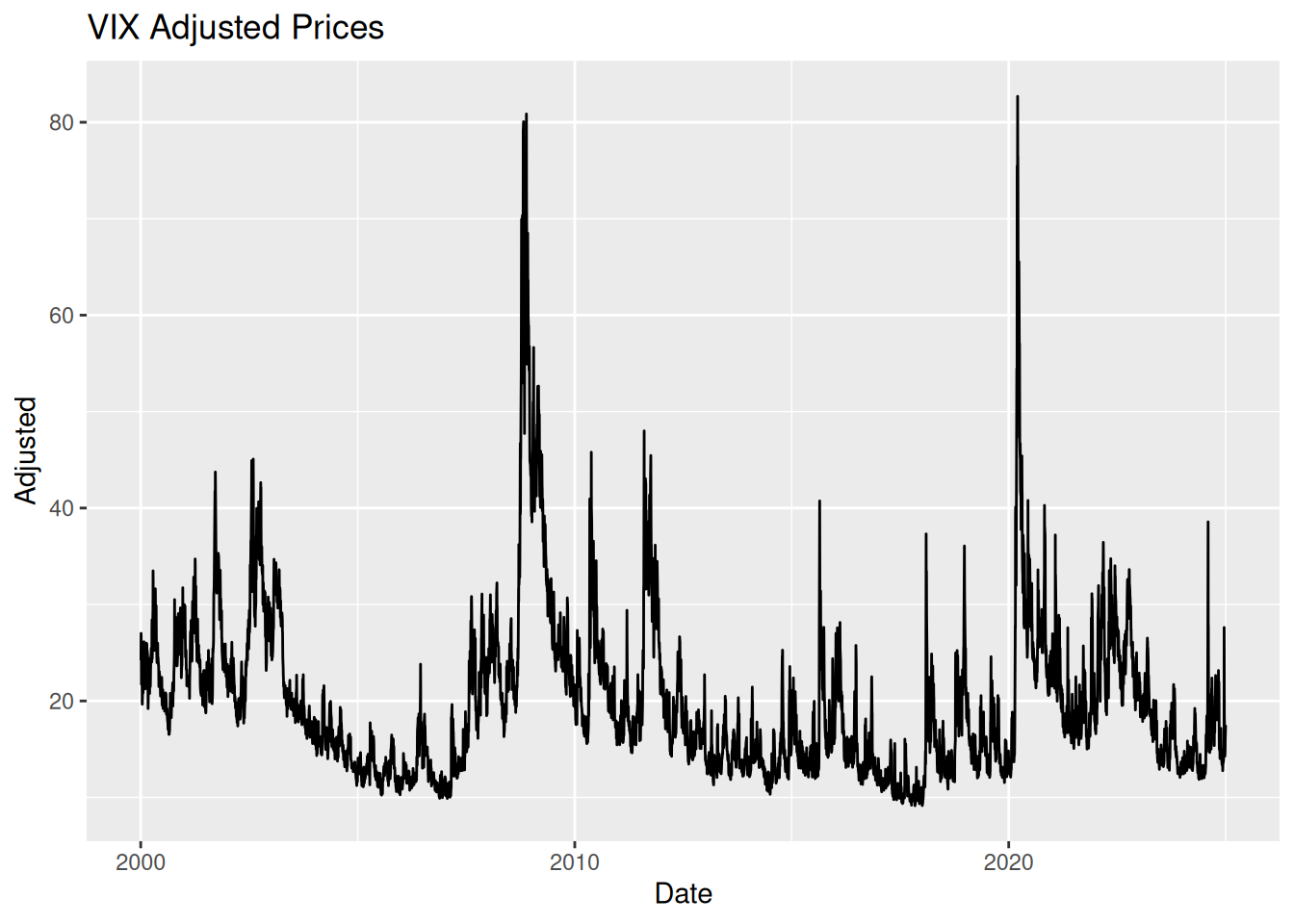

ACF and PACF Analysis

vix_data %>% 
  ACF(adjusted) %>% 
  autoplot() +
  labs(title = "ACF of VIX Data")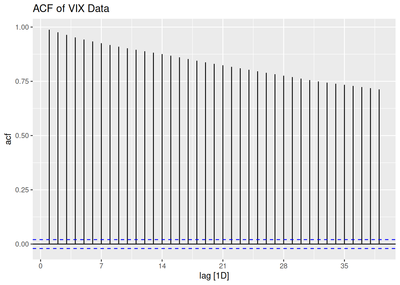

vix_data %>% 
  PACF(adjusted) %>% 
  autoplot() +
  labs(title = "PACF of VIX Data")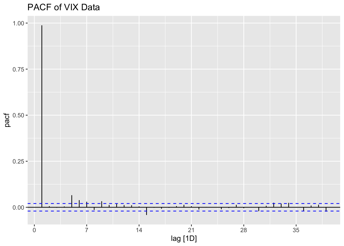

Observation:
The persistence in ACF suggests potential need for differencing, but we’ll let ARIMA automatically handle any required transformations through its \(d\) parameter.

Model Fitting Using Tidyverts

1. ARIMA Model (Original Series)

# Fit an ARIMA model on original series
model_arima <- vix_data %>% 
  model(ARIMA(adjusted))

# Display summary report
report(model_arima)

Series: adjusted 
Model: ARIMA(3,1,1)(0,0,2)[7] 

Coefficients:
         ar1     ar2      ar3      ma1    sma1    sma2
      0.9615  0.0082  -0.0179  -0.9811  0.0286  0.0553
s.e.  0.0168  0.0145   0.0122   0.0133  0.0115  0.0107

sigma^2 estimated as 1.728:  log likelihood=-15446.52
AIC=30907.05   AICc=30907.06   BIC=30956.88

# Display accuracy metrics
model_arima %>% accuracy()

# A tibble: 1 × 10
  .model          .type         ME  RMSE   MAE    MPE  MAPE  MASE RMSSE     ACF1
  <chr>           <chr>      <dbl> <dbl> <dbl>  <dbl> <dbl> <dbl> <dbl>    <dbl>
1 ARIMA(adjusted) Traini… -0.00181  1.31 0.731 -0.220  3.42 0.356 0.403 -2.97e-4

2. ETS Model

# Fit ETS model on original series
model_ets <- vix_data %>% 
  model(ETS(adjusted))

# Display summary report
report(model_ets)

Series: adjusted 
Model: ETS(M,Ad,M) 
  Smoothing parameters:
    alpha = 0.9998863 
    beta  = 0.0449181 
    gamma = 0.0001019892 
    phi   = 0.8178318 

  Initial states:
     l[0]       b[0]    s[0]     s[-1]     s[-2]    s[-3]     s[-4]     s[-5]
 25.49738 -0.7829361 1.00114 0.9990668 0.9956332 1.002539 0.9994978 0.9996608
    s[-6]
 1.002462

  sigma^2:  0.003

     AIC     AICc      BIC 
83569.41 83569.45 83661.96

# Display accuracy metrics
model_ets %>% accuracy()

# A tibble: 1 × 10
  .model        .type           ME  RMSE   MAE    MPE  MAPE  MASE RMSSE    ACF1
  <chr>         <chr>        <dbl> <dbl> <dbl>  <dbl> <dbl> <dbl> <dbl>   <dbl>
1 ETS(adjusted) Training -0.000342  1.32 0.732 -0.120  3.43 0.356 0.405 -0.0392

Forecasting with the Optimal Model

# Forecast 12 months ahead using ARIMA
forecast_arima <- model_arima %>% 
  forecast(h = "12 months")

# Plot forecast in original units
forecast_arima %>% 
  autoplot(vix_data) +
  labs(title = "12-Month VIX Forecast", y = "Adjusted VIX", x = "Date")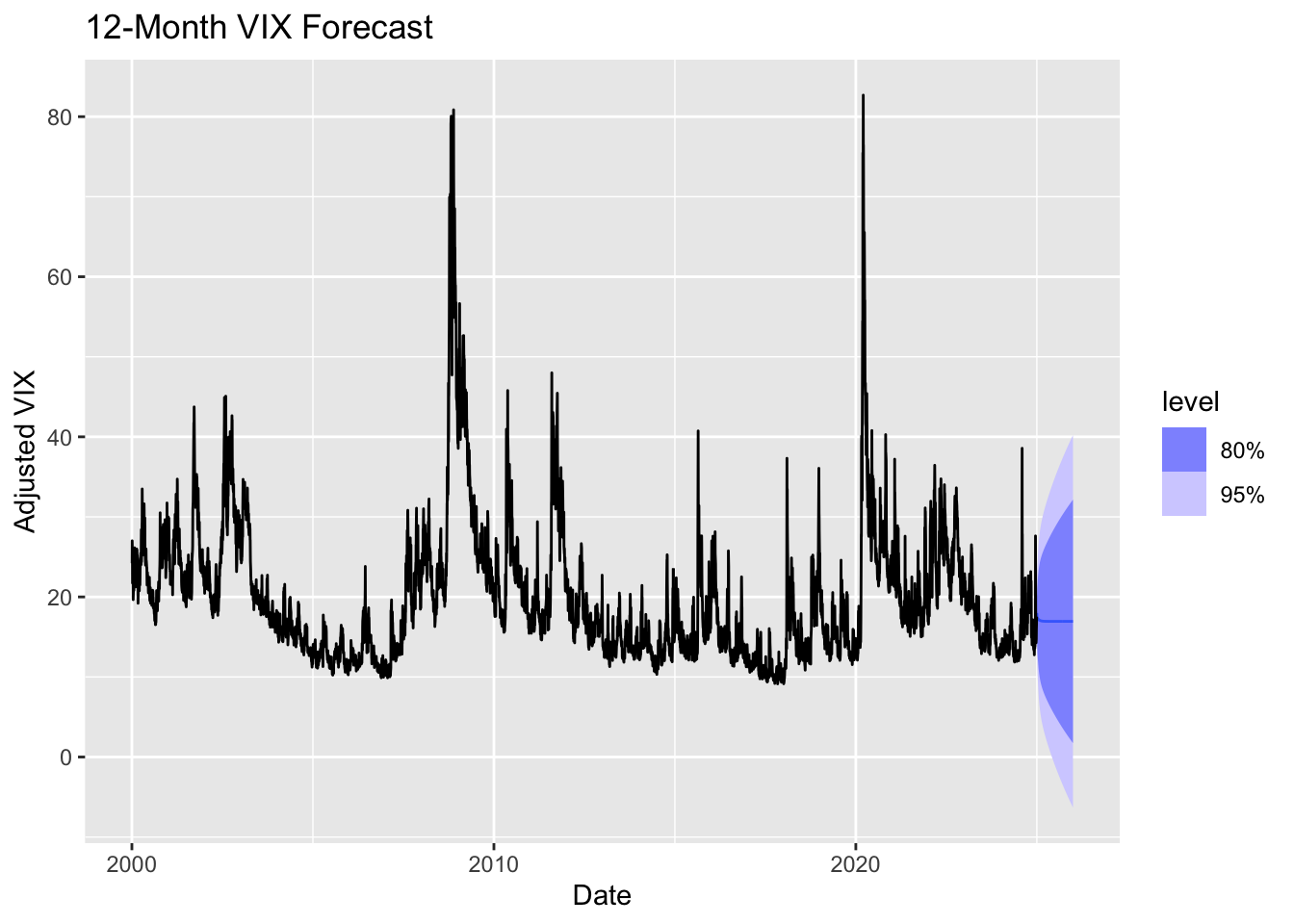

Lab Activity: Modeling Stock Returns with ARIMA

Model daily SPY returns using ARIMA, analyze residuals, and compare with ETS.

Tasks

Retrieve SPY data (2015-01-01 to present) and compute daily log returns
Perform EDA (time series plot, ACF/PACF)
Fit ARIMA(2,0,1) and ETS models to returns
Compare models using AIC and RMSE
Forecast 1-month ahead returns

Solution

# Task 1: Data Preparation
spy_data <- tq_get("SPY", from = "2015-01-01") %>% 
  as_tsibble(index = date) %>% 
  tsibble::fill_gaps() %>% 
  mutate(adjusted = na.approx(adjusted),
         log_return = difference(log(adjusted))) %>% 
  select(date, adjusted, log_return) %>% 
  tidyr::drop_na()


# Task 2: EDA
spy_data %>% autoplot(log_return) +
  labs(title = "SPY Daily Log Returns", y = "Return")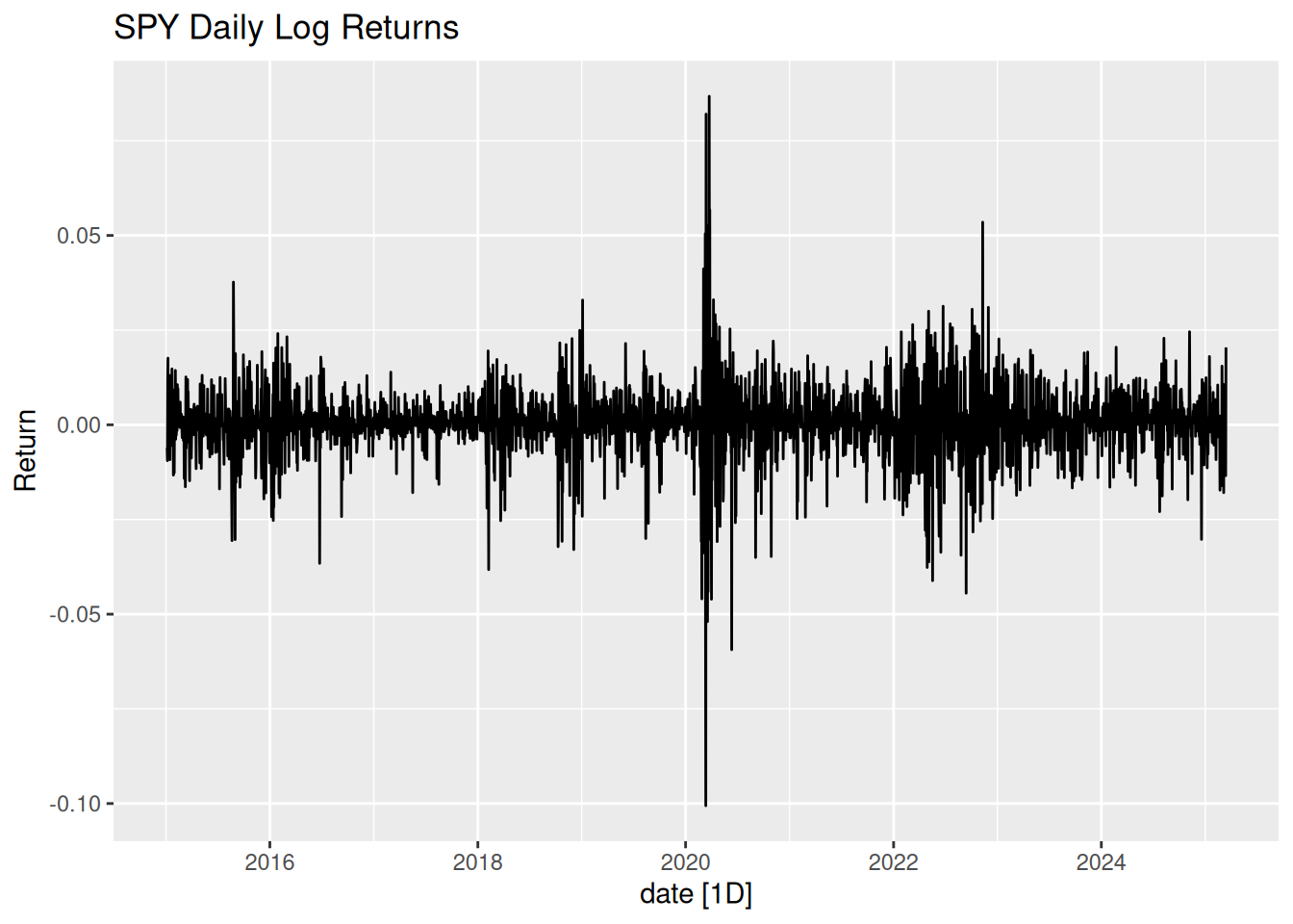

spy_data %>% ACF(log_return) %>% autoplot()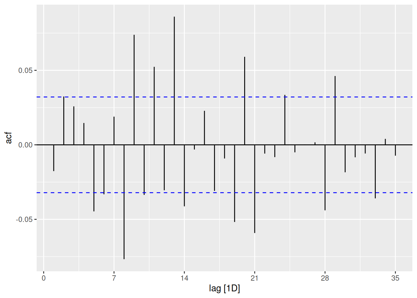

spy_data %>% PACF(log_return) %>% autoplot()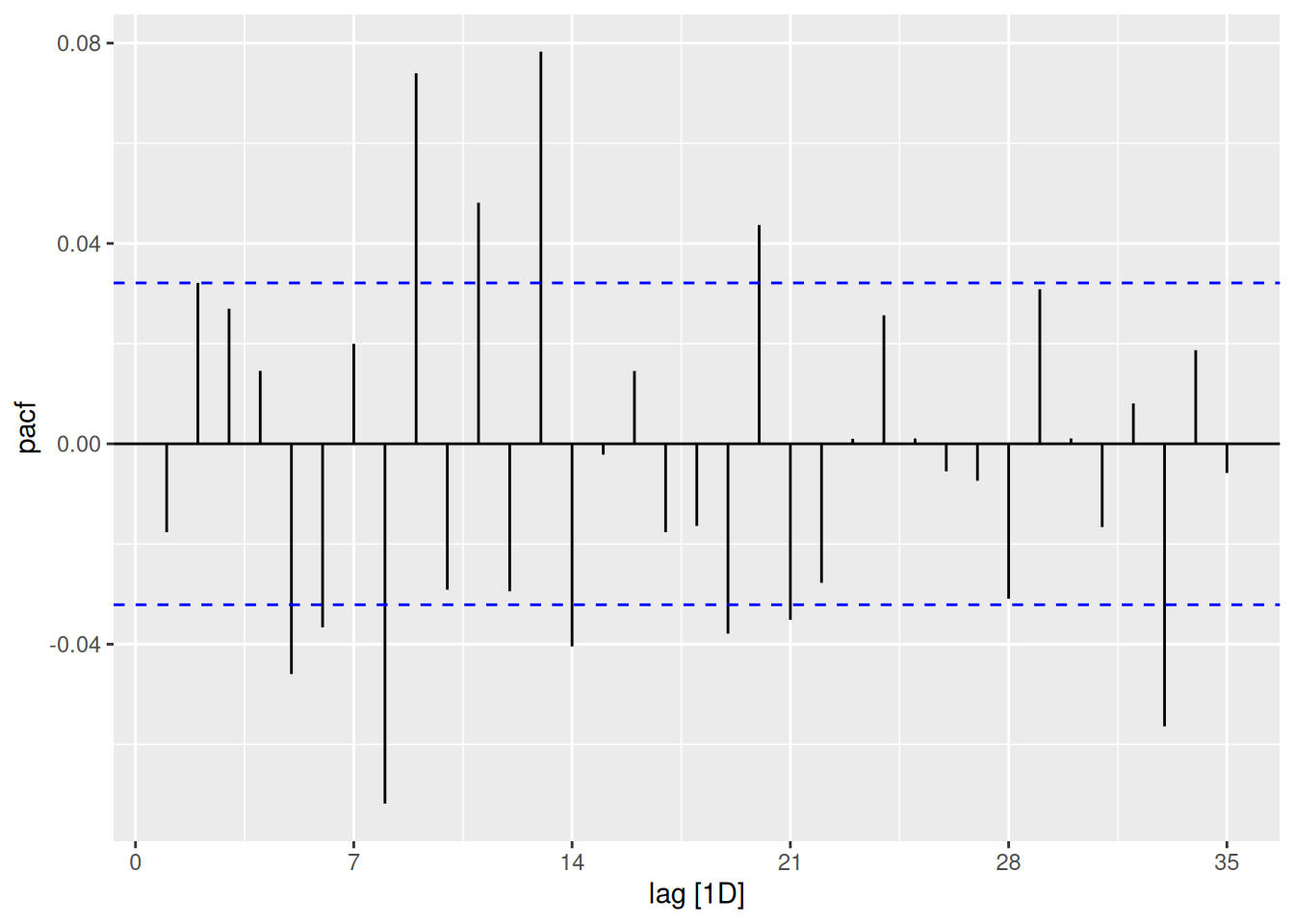

# Task 3: Model Fitting
fit_arima <- spy_data %>% 
  model(ARIMA(log_return ~ pdq(2,0,1)))

fit_ets <- spy_data %>% 
  model(ETS(log_return))

# Task 4: Model Comparison
glance(fit_arima) %>% select(AIC, AICc, BIC)

# A tibble: 1 × 3
      AIC    AICc     BIC
    <dbl>   <dbl>   <dbl>
1 -24976. -24976. -24926.

glance(fit_ets) %>% select(AIC, AICc, BIC)

# A tibble: 1 × 3
     AIC   AICc    BIC
   <dbl>  <dbl>  <dbl>
1 -4714. -4714. -4695.

accuracy(fit_arima)

# A tibble: 1 × 10
  .model         .type       ME    RMSE     MAE   MPE  MAPE  MASE RMSSE     ACF1
  <chr>          <chr>    <dbl>   <dbl>   <dbl> <dbl> <dbl> <dbl> <dbl>    <dbl>
1 ARIMA(log_ret… Trai… -6.56e-7 0.00866 0.00511   NaN   Inf 0.697 0.722 -4.23e-4

accuracy(fit_ets)

# A tibble: 1 × 10
  .model          .type       ME    RMSE     MAE   MPE  MAPE  MASE RMSSE    ACF1
  <chr>           <chr>    <dbl>   <dbl>   <dbl> <dbl> <dbl> <dbl> <dbl>   <dbl>
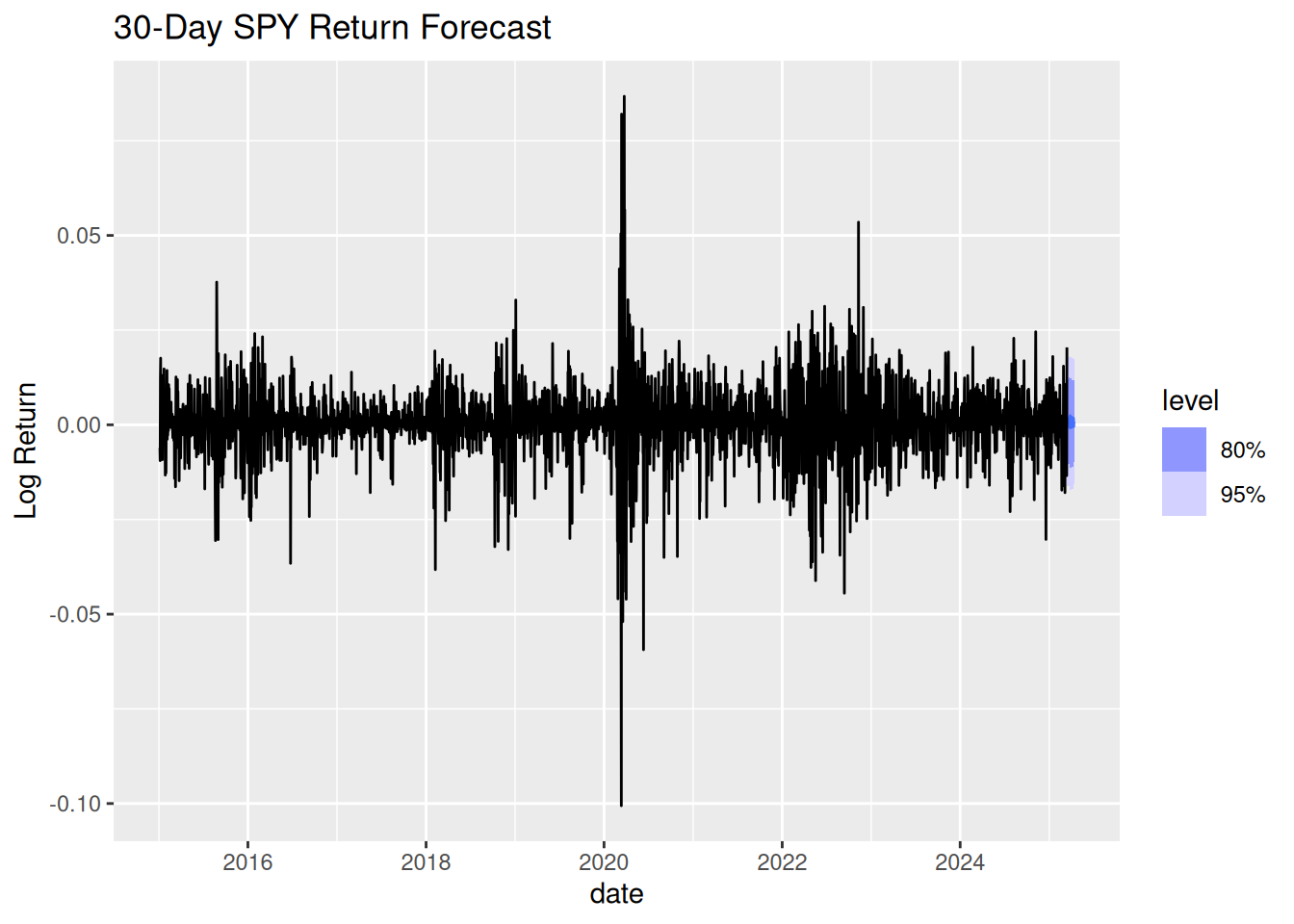
1 ETS(log_return) Train… 1.60e-6 0.00870 0.00509  -Inf   Inf 0.695 0.726 -0.0305

# Task 5: Forecasting
fit_arima %>% 
  forecast(h = 30) %>% 
  autoplot(spy_data) +
  labs(title = "30-Day SPY Return Forecast", y = "Log Return")