production_data <- aus_production %>%
  dplyr::select(Quarter, Beer, Gas, Electricity) %>%
  drop_na() %>%
mutate(across(c(Beer, Gas, Electricity), log))Activity36
Extending to Multiple Variables with Structural Breaks
Data Prep: Australian Production (Beer, Gas, Electricity)
Activity 1: Detecting Structural Breaks
Structural Break Detection
Using Chow test and CUSUM for regime shifts:
# 1. Visual break identification
production_data %>%
  pivot_longer(-Quarter) %>%
  autoplot(value) +
  geom_vline(
    xintercept = as.numeric(yearquarter("1968 Q3")),
    color = "firebrick",
    linetype = 2
  ) +
  labs(title = "Production Trends with Suspected Structural Break")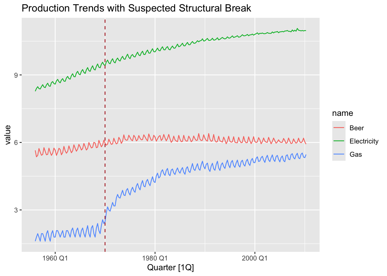
# 2. Formal breakpoints test
library(strucchange)
bp_test <- Fstats(Beer ~ Gas + Electricity, data = production_data)
break_date <- breakpoints(bp_test)$breakpoints %>%
  production_data$Quarter[.]
Handling Structural Breaks
Create intervention dummy:
# Create an intervention dummy: 0 before break, 1 after break
production_data <- production_data %>%
  mutate(regime = if_else(Quarter >= break_date, 1, 0))
Activity 2: ARIMA with an Intervention Dummy
Incorporating the intervention variable as an external regressor.
# Fit ARIMA model with intervention dummy using xreg()
arima_model <- production_data %>%
  model(ARIMA(Beer ~ xreg(regime)))

report(arima_model)
Series: Beer
Model: LM w/ ARIMA(3,0,1)(0,1,1)[4] errors
Coefficients:
ar1 ar2 ar3 ma1 sma1 regime
0.4114 0.3476 0.2172 -0.3827 -0.7269 -0.0156
s.e. 0.1396 0.0774 0.1078 0.1339 0.0541 0.0216
sigma^2 estimated as 0.001226: log likelihood=415.13
AIC=-816.25 AICc=-815.71 BIC=-792.69arima_model %>% tidy() %>% filter(term == "regime")# A tibble: 1 × 6
.model term estimate std.error statistic p.value
<chr> <chr> <dbl> <dbl> <dbl> <dbl>
1 ARIMA(Beer ~ xreg(regime)) regime -0.0156 0.0216 -0.724 0.470The underlying model is represented as
\[ \begin{align} y_t &= \mu + \sum_{i=1}^{p}\phi_i y_{t-i} + \sum_{j=1}^{q}\theta_j \epsilon_{t-j} + \beta D_t + \epsilon_t, \end{align} \]
where \(D_t\) is defined as
\[ D_t = \begin{cases} 0, & t < \text{break date}, \\ 1, & t \geq \text{break date}, \end{cases} \]
Activity 3: ETS Models on Regime-Split Data
Since ETS models do not natively accept exogenous regressors, we split the data into pre- and post-break regimes and fit separate ETS models.
# Split the data based on break_date
data_pre_break <- production_data %>% filter(Quarter < break_date)
data_post_break <- production_data %>% filter(Quarter >= break_date)

# Fit ETS models for Beer production on each regime
ets_pre <- data_pre_break %>% model(ETS(Beer))
ets_post <- data_post_break %>% model(ETS(Beer))

# Output summaries
report(ets_pre)
Series: Beer
Model: ETS(A,A,A)
Smoothing parameters:
alpha = 0.09973697
beta = 0.03911698
gamma = 0.0001004978
Initial states:
l[0] b[0] s[0] s[-1] s[-2] s[-3]
5.539214 0.0006337494 0.1727994 -0.07509174 -0.1381876 0.04047987
sigma^2: 0.0012
AIC AICc BIC
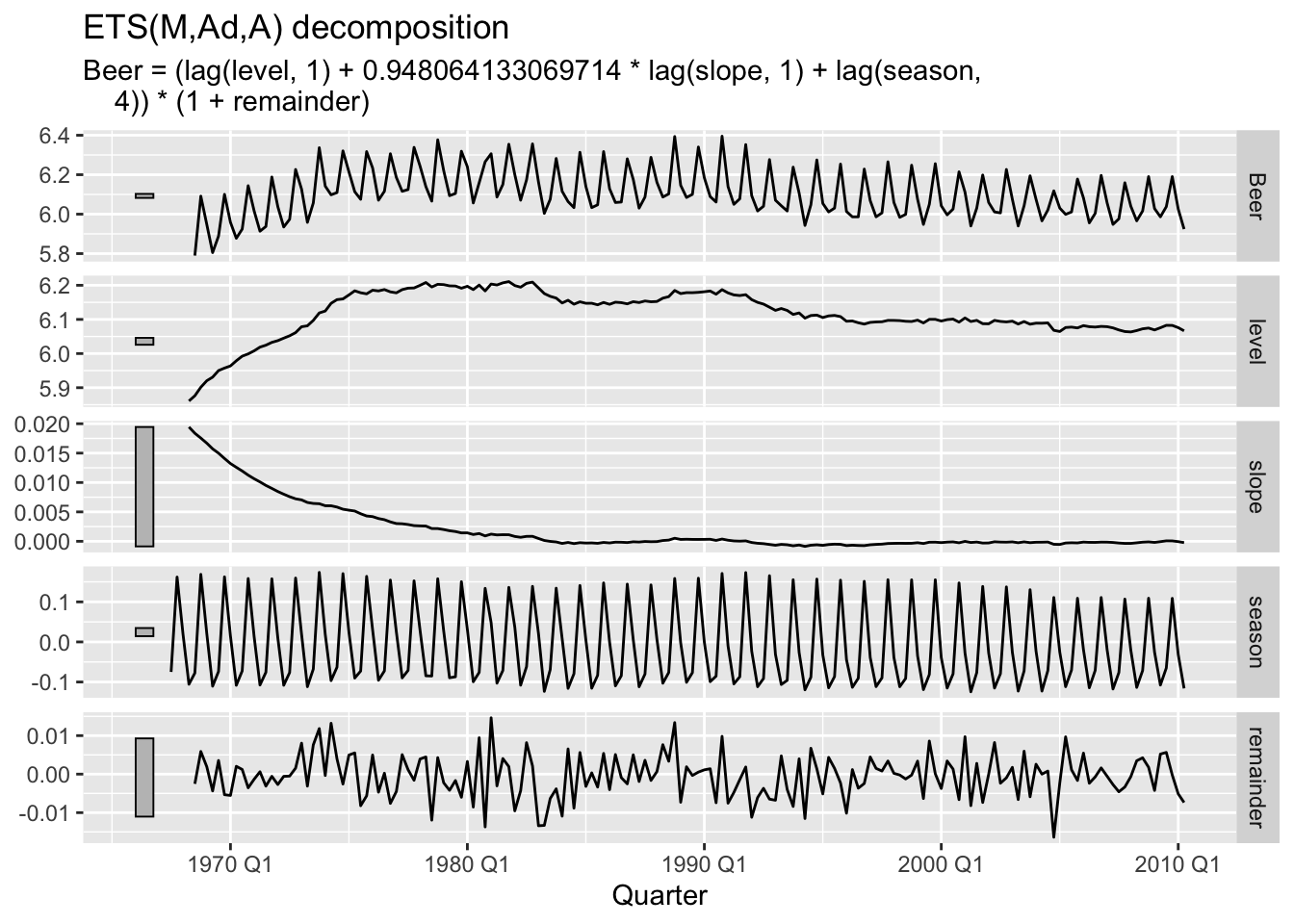
-132.8992 -128.3992 -115.6910 report(ets_post)Series: Beer
Model: ETS(M,Ad,A)
Smoothing parameters:
alpha = 0.2117282
beta = 0.003866127
gamma = 0.1908595
phi = 0.9480641
Initial states:
l[0] b[0] s[0] s[-1] s[-2] s[-3]
5.86103 0.01944297 -0.1056501 0.01861439 0.1619088 -0.07487303
sigma^2: 0
AIC AICc BIC
-249.0023 -247.6010 -217.7627 ets_pre %>%
components() %>%
autoplot()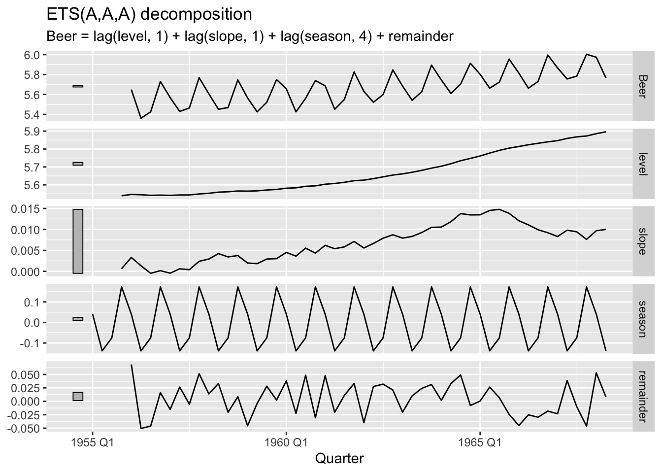
ets_post %>%
  components() %>%
  autoplot()