Activity4

1. MA(1) Process

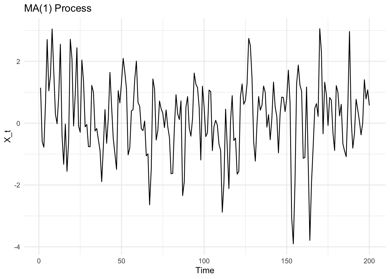
The Moving Average of Order 1 (MA(1)) process is defined as:

\[ X_t = \varepsilon_t + \theta \varepsilon_{t-1} \]
where \(\varepsilon_t\) is white noise with variance \(\sigma^2\).

Key Properties:

• Short Memory: The autocorrelation function (ACF) cuts off after lag 1.
  
• Variance: \(\gamma(0) = \sigma^2(1 + \theta^2)\).
  
• Covariance: \(\gamma(1) = \theta \sigma^2\).

Simulation in R:

# MA(1) simulation
n <- 200
theta <- 0.8
eps <- rnorm(n + 1)  # ε_0 to ε_n
ma_values <- numeric(n)
for(t in 1:n) {
  ma_values[t] <- eps[t+1] + theta*eps[t]  # X_t = ε_t + θε_{t-1}
}

ma1 <- tsibble(time = 1:n, y = ma_values, index = time)
# Plot
ggplot(ma1, aes(x = time, y = y)) +
  geom_line() +
  labs(title = "MA(1) Process", x = "Time", y = "X_t") +
  theme_minimal()

---

2. AR(1) Process

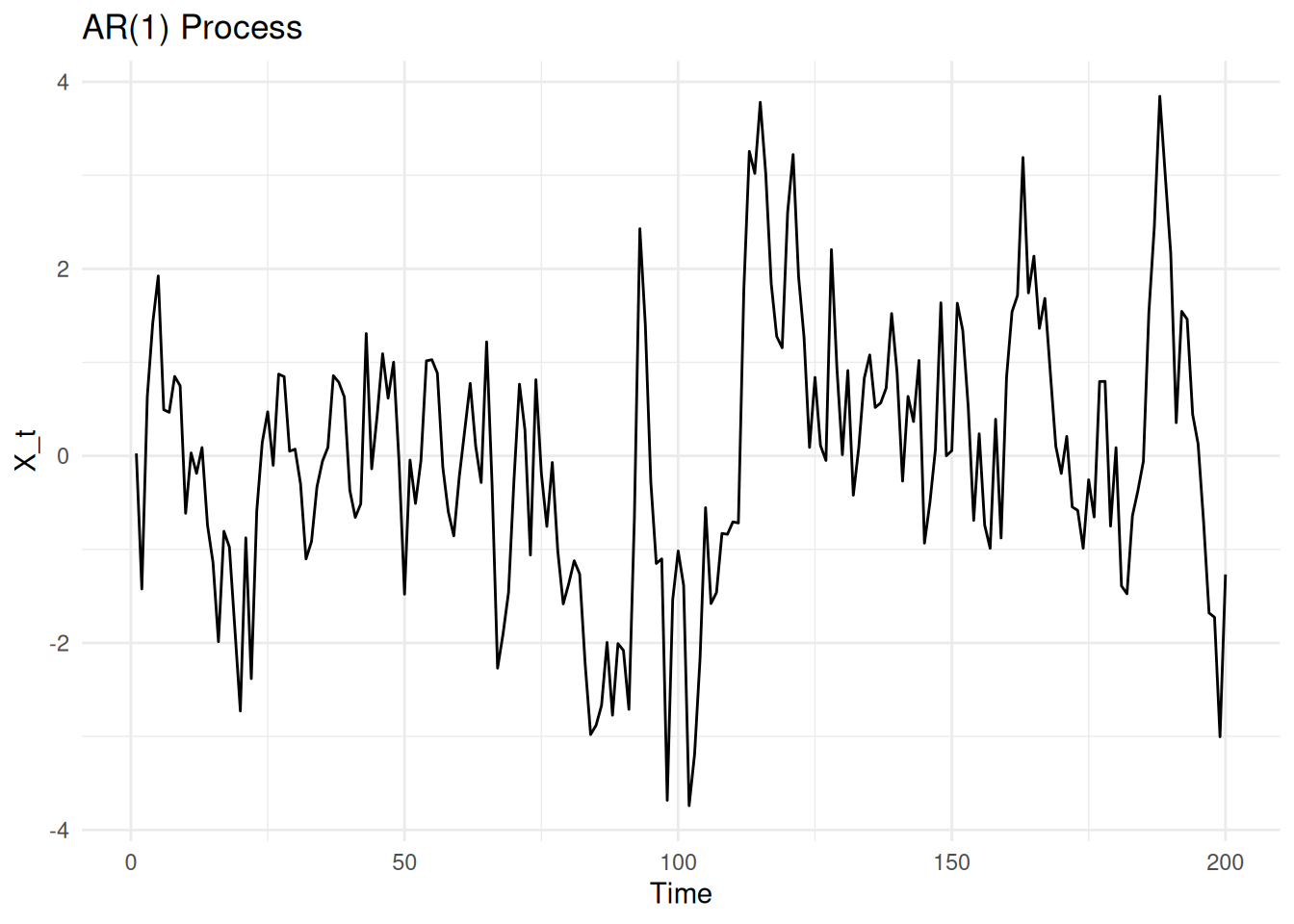
The Autoregressive of Order 1 (AR(1)) process is defined as:

\[ X_t = \phi X_{t-1} + \varepsilon_t \]
where \(\varepsilon_t\) is white noise with variance \(\sigma^2\).

Key Properties:

• Stationarity: Requires \(|\phi| < 1\).
  
• ACF: Decays exponentially as \(\rho(k) = \phi^k\).
  
• PACF: Cuts off after lag 1.

Simulation in R:

# AR(1) simulation
n <- 200
phi <- 0.8
eps <- rnorm(n)
ar_values <- numeric(n)
ar_values[1] <- eps[1]  # X_1 = ε_1
for(t in 2:n) {
  ar_values[t] <- phi*ar_values[t-1] + eps[t]
}

ar1 <- tsibble(time = 1:n, y = ar_values, index = time)
# Plot
ggplot(ar1, aes(x = time, y = y)) +
  geom_line() +
  labs(title = "AR(1) Process", x = "Time", y = "X_t") +
  theme_minimal()

---

3. Random Walk with Drift

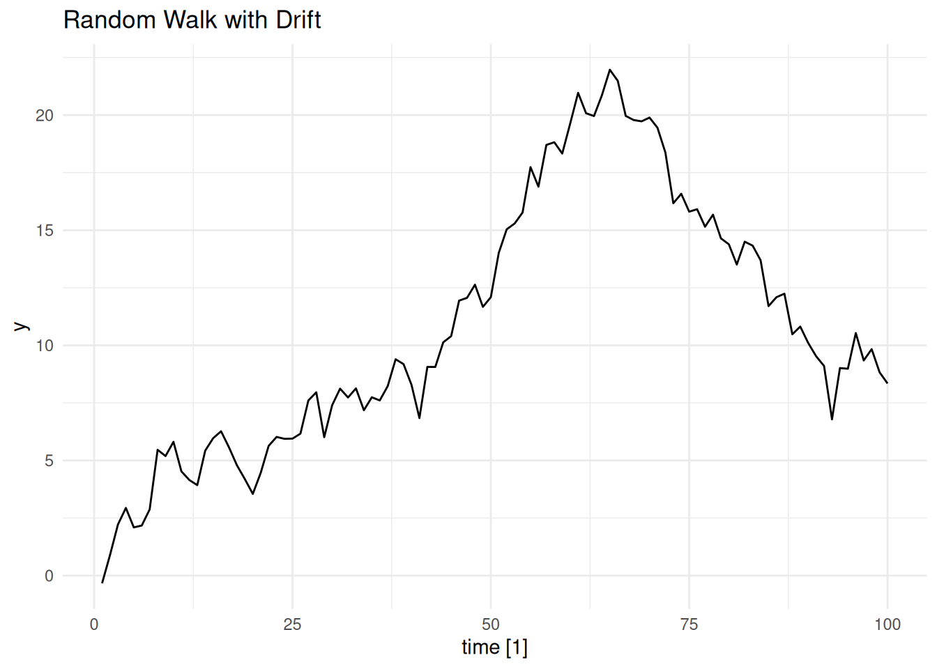
The Random Walk with Drift is defined as:

\[ X_t = \delta + X_{t-1} + \varepsilon_t \]
where \(\varepsilon_t\) is white noise with variance \(\sigma^2\), and \(\delta\) is the drift term.

Key Characteristics:

• Non-Stationarity: Variance grows with time, \(\operatorname{Var}(X_t) = t \sigma^2\).

Simulation in R:

library(tsibble)
library(feasts)

# Random Walk with Drift simulation
n <- 100
delta <- 0.1
rw_values <- cumsum(delta + rnorm(n))  # Cumulative sum of (δ + ε_t)

rw_drift <- tsibble(time = 1:n, y = rw_values, index = time)
autoplot(rw_drift, y) + labs(title = "Random Walk with Drift") +
  theme_minimal()

Lab Activity: More Simulations and Comparisons

Q1: MA(1) Process

Prompt: Simulate and visualize an MA(1) process with parameter θ = 0.9 using tsibble and autoplot.

Solution:

Q2: AR(1) Process

Prompt: Simulate and visualize an AR(1) process with parameter \(\phi=0.96\) using tsibble and autoplot.

Solution:

Q3: Random Walk & Comparison

Prompt: Create a random walk with drift \((\delta = 0.2)\), then visualize all three processes together.

Solution: